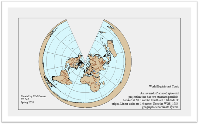
Mapping the World

I downloaded the dataset from the homework assignment and proceeded to create a personalized map of the world. I added the “World Continents” data to create a nice base upon which to build. Given my focus on water resources, I also added “rivers” and “lakes”. If you choose to add these same datasets, you will notice that the label for river systems stays the same once it’s added to the Table of Contents but the label for “lakes” changes to “World Lakes”. For the sake of consistency, I changed the label name to “World Rivers”. After I selected the data that I wanted to use, I changed the symbology for each one. I changed my projection to World Equidistant Conic. This is a conic secant projection that cuts through the surface of the earth resulting in two standard parallels. It also provides us with a view of the earth we are unaccustomed to seeing.

Mapping the United States

I created my map of the United States using the default coordinate system and adding the U.S. States data as well as the Major Cities data. I then built a query by accessing the Layer Properties (right click “Capital Cities”), clicking the Definition Query tab, and clicking Query Builder. Double click CAPITAL, hit the = sign once, click “get Unique Values”, double-click ‘Y’ and don’t forget to Verify to ensure the query functions. Once you get the all clear, hit OK then Apply. Major US cities that are not the capital will disappear to clean up the map a little bit. Next, we want to determine the latitude and longitude of three major cities.

First, I want to use a measurement with which I am more familiar so I clicked on “View”, scrolled down to “Data Frame Properties”, and used the drop-down menu for “Display” to “Degrees Minutes Seconds”. Next, I’ll change my cursor to “Identify” from the toolbar and when I click on a city, the latitude and longitude will appear. Austin, TX is located at (-97.795136, 30.377267), Sacramento, CA is located at (-121.473153, 38.563802), and Juneau, AK is located at (-134.136644, 58.397800).

I went into the Symbology for U.S. States and changed their color to blue. You may need to increase the Outline Width to 1.00 and give it a color to ensure you can see the state lines, I chose to make the state lines white. I changed the symbol for the capitals to stars, made them red, proportional to their population sizes, adjusted the size so that the stars weren’t too big, and divided them into 5 classes.

I took a measurement of the distance from Olympia, WA to August, MA. The measurement in the original coordinate system was 3,066.766 miles. I then changed the coordinate system to USA Albers Equal Area projection and re-measured the distance. This time, the distance measured was 652.148 miles (1,049.530471 kilometers).

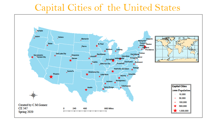
Next, we want to identify the two cities with the largest population and the highest elevation. Right click the “Capital Cities” layer, then click on Attribute Table. Extend the Attribute Table to see all the data we have, right click on “POP1990” and click “Sort Descending” to see the capital with the most people. The most populated capital city in 1990 was Phoenix, AZ with 983,403 people and the least populated city is Montpelier, VT with 8,247 residents. Next, click on “Elevation” and “Sort Descending”. The capital city at the highest elevation is Santa Fe, New Mexico. Scrolling to the bottom of the Attribute Table we see that several U.S. cities have a -99 elevation. I originally thought that perhaps these cities were below sea level but a quick Google search proved otherwise. I determined that there simply wasn’t data for these cities and that is why they all have the same quantity of -99.

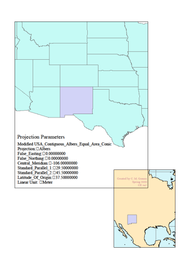
Mapping New Mexico

Lastly, we want to focus on our home state of New Mexico. You’ll want to export the state directly from the geodatabase by clicking on the “Select Features” tool from the toolbar at the top, clicking on the state of New Mexico, and then right clicking the layer “U.S. States”. Choose the “Data” option and click on “Export Data” when it appears. You are now exporting the data for the state of New Mexico onto your preferred location, in my case it’s the flashdrive I store all my work on. You may need to connect to your preferred folder once more if you are using the school’s computers which you can do with the ArcCatalog program.

Once you have New Mexico on the map, you’ll want to change the coordinate system to Albers and set the central meridian to 106. We won’t be using the DataFrame Properties for this, we’ll be using the ArcToolbox. Click on ArcToolbox at the top, Navigate to “Data Management Tools”, click on “Projections and Transformations”, then click the little hammer with “Project” next to it. Remember, when you see “project” in ArcGIS it’s referring to a projection not a project. Enter the name of the feature you are working with, if you haven’t changed the name to New Mexico it will likely be “Export_Output”. Click on the little hand pointing to a place on a paper to access the “Spatial Reference Properties”. I used the seach bar at the top to search for “Albers” (it is located in Projected Coordinate Systems>North America). Right click on “USA Contiguous Albers Equal Area Conic” and select “Copy and Modify”. This will open “Projected Coordinate System Properties”. In the box for Central Meridian, enter “-106”.

Create your desired layout including the projection parameters.