METHODS

I chose to examine the effects of this fire on the impacted watersheds as seen in Figure 1. The land impacted by the fire is shown in red, near the area labeled Los Alamos. This background map came from Assignment 2 which dealt with Pan Evaporation data. I used the county data in order to create a vicinity map for the fire data. The fire data came from the Burned Area Emergency Response (BAER) process through the US Forest Service. This data was created specifically for soil analysis and was last updated in 2014. Lastly, the digital elevation model (DEM) used for this analysis came from the US Geological Survey (USGS) from the National Map. It is a 1/3 arc-second DEM, which is approximately 10m by 10m. This data was all analyzed using ArcGIS 10.6.1.

Since this analysis involves New Mexico alone, the maps are all projected using NAD 1983, UTM Zone 13N so that New Mexico is centered on the map. This projection method minimizes area distortion and distance distortion which are both important for the stream length analysis. Using the same projection for all data makes it possible to overlay layers and compare distances, or shapes without distortion.

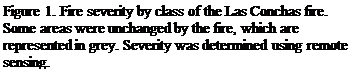
The fire data categorized the severity of the Las Conchas fire into three categories, determined by the loss of organic matter in the soil (Keeley, 2009). This analysis was done by BAER using remote 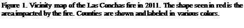Text Box: Figure 1. Vicinity map of the Las Conchas fire in 2011. The shape seen in red is the area impacted by the fire. Counties are shown and labeled in various colors. sensing to determine the amount of organic matter remaining post-burn. These categories are shown in Figure 2, with the darkest color representing the highest severity class. Some areas of the fire were unchanged, and these areas were left out of the analysis.

Text Box: Figure 2. Fire severity by class of the Las Conchas fire. Some areas were unchanged by the fire, which are represented in grey. Severity was determined using remote sensing. A watershed was established using the DEM taken from the National Map from the USGS website and the hydrology toolset from ArcToolbox. A model of the steps taken to determine the streams and watershed is shown to the left in Figure 3. New layers were created from each fire severity class in order to overlay the stream layer with the different categories of burn areas. The length of impacted stream for each category was determined using raster calculator with these individual layers (Figure 4).

Text Box: Figure 3. A model of the steps taken to determine the stream network that flows through the affected area in northern New Mexico, created using the model builder in ArcGIS.