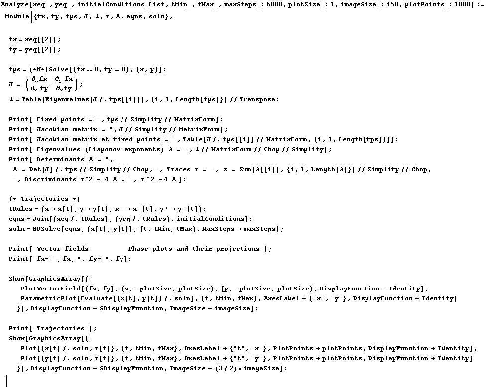
General 2D Dynamical Systems with application to van der Pol dynamics

General System Trajectories

<<Graphics`PlotField`

Dynamical 2D System Trajectories: Steven H. Strogatz Nonlinear dynamics and Chaos, Westview Pess, 1994 Example7.6.3 two-timing (two time scale) analysis of the van der Pol oscillator

For DS of the form x'=ax+by, y'=cx+dy, the (only) fixed point is at the origin {0,0}.

xeq = x ' == y ;

yeq = y ' == -x - μ * (x^2 - 1) * y ;

Print[StyleForm["Equations of motion: ", FontSize→14, FontWeight→"Bold"], {xeq, yeq}//ColumnForm]

Print[StyleForm["Two-timing envelope function: ", FontSize→14, FontWeight→"Bold"], r[t_] = 2/Sqrt[1 + 3E^(-μ * t)]]

Equations of motion:  {{x^′y}, {y^′ -x - (x^2 - 1) y μ}}

Two-timing envelope function: 2/(1 + 3 ^(-t μ))^(1/2)

Stragatz Example7.6.3

Print["Nonlinear damping parameter μ = ", μ = 0.1] ;

Print["Initial conditions: ", initialConditions = {x[0] == 1, y[0] == 0}] ;

Print["\nAnalysis"] ;

Analyze[xeq, yeq, initialConditions, 0, 16Pi]

Nonlinear damping parameter μ = 0.1

Initial conditions:  {x(0) 1, y(0) 0}

<br />Analysis

Fixed points =  ( {{y→0., x→0.}} )

Jacobian matrix =  ( {{0, 1}, {-0.2 x y - 1, 0.1 - 0.1 x^2}} )

Jacobian matrix at fixed points =  {( {{0, 1}, {-1., 0.1}} )}

Eigenvalues (Liaponov exponents) λ =  ( {{0.05 + 0.998749 }, {0.05 - 0.998749 }} )

Determinants Δ =  {1.} , Traces τ =  {0.1} , Discriminants τ^2 - 4 Δ =  {-3.99}

Vector fields          Phase plots and their projections

fx= y, fy=  -x - 0.1 (x^2 - 1) y

[Graphics:HTMLFiles/2DDSVDP_23.gif]

Trajectories

[Graphics:HTMLFiles/2DDSVDP_25.gif]

Strogatz Example7.6.3 van der Pol oscillator with longer time range

Print["Nonlinear damping parameter μ = ", μ = 0.1] ;

Print["Initial conditions: ", initialConditions = {x[0] == 1, y[0] == 0}] ;

Print["\nAnalysis"] ;

Analyze[xeq, yeq, initialConditions, 0, 50Pi]

Nonlinear damping parameter μ = 0.1

Initial conditions:  {x(0) 1, y(0) 0}

<br />Analysis

Fixed points =  ( {{y→0., x→0.}} )

Jacobian matrix =  ( {{0, 1}, {-0.2 x y - 1, 0.1 - 0.1 x^2}} )

Jacobian matrix at fixed points =  {( {{0, 1}, {-1., 0.1}} )}

Eigenvalues (Liaponov exponents) λ =  ( {{0.05 + 0.998749 }, {0.05 - 0.998749 }} )

Determinants Δ =  {1.} , Traces τ =  {0.1} , Discriminants τ^2 - 4 Δ =  {-3.99}

Vector fields          Phase plots and their projections

fx= y, fy=  -x - 0.1 (x^2 - 1) y

[Graphics:HTMLFiles/2DDSVDP_40.gif]

Trajectories

[Graphics:HTMLFiles/2DDSVDP_42.gif]

van der Pol oscillator with smaller damping parameter μ

Print["Nonlinear damping parameter μ = ", μ = 0.01] ;

Print["Initial conditions: ", initialConditions = {x[0] == 1, y[0] == 0}] ;

Print["\nAnalysis"] ;

Analyze[xeq, yeq, initialConditions, 0, 50Pi]

Nonlinear damping parameter μ = 0.01

Initial conditions:  {x(0) 1, y(0) 0}

<br />Analysis

Fixed points =  ( {{y→0., x→0.}} )

Jacobian matrix =  ( {{0, 1}, {-0.02 x y - 1, 0.01 - 0.01 x^2}} )

Jacobian matrix at fixed points =  {( {{0, 1}, {-1., 0.01}} )}

Eigenvalues (Liaponov exponents) λ =  ( {{0.005 + 0.999987 }, {0.005 - 0.999987 }} )

Determinants Δ =  {1.} , Traces τ =  {0.01} , Discriminants τ^2 - 4 Δ =  {-3.9999}

Vector fields          Phase plots and their projections

fx= y, fy=  -x - 0.01 (x^2 - 1) y

[Graphics:HTMLFiles/2DDSVDP_57.gif]

Trajectories

[Graphics:HTMLFiles/2DDSVDP_59.gif]

van der Pol oscillator with larger damping parameter μ

Print["Nonlinear damping parameter μ = ", μ = 1.] ;

Print["Initial conditions: ", initialConditions = {x[0] == 1, y[0] == 0}] ;

Print["\nAnalysis"] ;

Analyze[xeq, yeq, initialConditions, 0, 50Pi]

Nonlinear damping parameter μ = 1.

Initial conditions:  {x(0) 1, y(0) 0}

<br />Analysis

Fixed points =  ( {{y→0., x→0.}} )

Jacobian matrix =  ( {{0, 1}, {-2. x y - 1, 1. - 1. x^2}} )

Jacobian matrix at fixed points =  {( {{0, 1}, {-1., 1.}} )}

Eigenvalues (Liaponov exponents) λ =  ( {{0.5 + 0.866025 }, {0.5 - 0.866025 }} )

Determinants Δ =  {1.} , Traces τ =  {1.} , Discriminants τ^2 - 4 Δ =  {-3.}

Vector fields          Phase plots and their projections

fx= y, fy=  -x - 1. (x^2 - 1) y

[Graphics:HTMLFiles/2DDSVDP_74.gif]

Trajectories

[Graphics:HTMLFiles/2DDSVDP_76.gif]

van der Pol oscillator with large damping parameter μ

Print["Nonlinear damping parameter μ = ", μ = 2.5] ;

Print["Initial conditions: ", initialConditions = {x[0] == 1, y[0] == 0}] ;

Print["\nAnalysis"] ;

Analyze[xeq, yeq, initialConditions, 0, 50Pi]

Nonlinear damping parameter μ = 2.5

Initial conditions:  {x(0) 1, y(0) 0}

<br />Analysis

Fixed points =  ( {{y→0., x→0.}} )

Jacobian matrix =  ( {{0, 1}, {-5. x y - 1, 2.5 - 2.5 x^2}} )

Jacobian matrix at fixed points =  {( {{0, 1}, {-1., 2.5}} )}

Eigenvalues (Liaponov exponents) λ =  ( {{2.}, {0.5}} )

Determinants Δ =  {1.} , Traces τ =  {2.5} , Discriminants τ^2 - 4 Δ =  {2.25}

Vector fields          Phase plots and their projections

fx= y, fy=  -x - 2.5 (x^2 - 1) y

[Graphics:HTMLFiles/2DDSVDP_91.gif]

Trajectories

[Graphics:HTMLFiles/2DDSVDP_93.gif]


Created by Mathematica  (December 1, 2009) Valid XHTML 1.1!