Weather Radar (NEXRAD) and Gage Station Precipitation Correlations

Applications of ArcGIS to a problem in hydrometeorology.

Kevin Scales

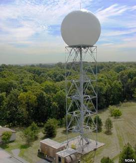
The current generation of Doppler Weather radar, the WSR-88D system, provides nearly continuous coverage of atmospheric liquid and solid phase water in the atmosphere. You may have seen a tower nearby.

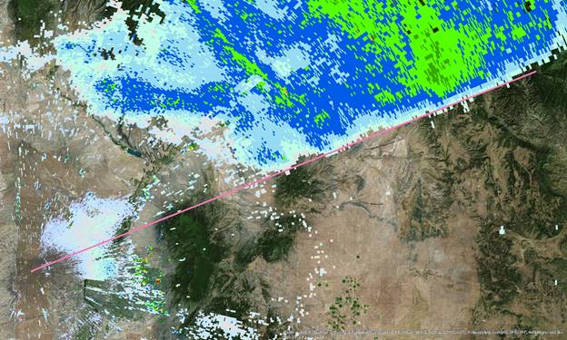
In Northwest New Mexico, the KABX station (not the one pictured above) provides coverage over a good portion of that section of the state.

The red lines, you may notice, are Interstates 40 and 25 with Albuquerque in the middle.

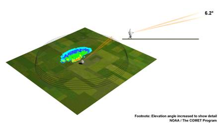
The radar system sweeps over multiple elevations to get a good 2-D and somewhat rough but decent 3-D picture

of the surrounding hydrometeors (a fancy term for raindrops, snowflakes, or hailstones).

Atmospheric refraction can bend the beam, causing it to return signals reflected from the ground, as if they were in the sky.

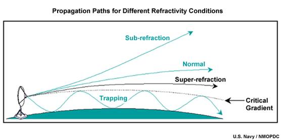
The beam can also be blocked. The Sandia range to the immediate east of Albuquerque provides a good example of this.

That straight edge in the snow and rain is not natural, or even actually there. The line along the top of Sandia crest tells us what’s been cut.

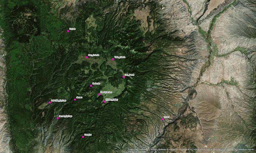
With ArcMap, we can show the study region of interest to us in and around the Valles Caldera and the

surrounding Jemez Forest. There are twelve gage stations run by the National Park Service, the sponsors of this work.

The tools available from the National Oceanic and Atmospheric Administration (NOAA) allow us to take radar data and convert it to

shape files readable by ArcGIS software. (They don’t do all the work for us, though. That color bar has to be created manually.

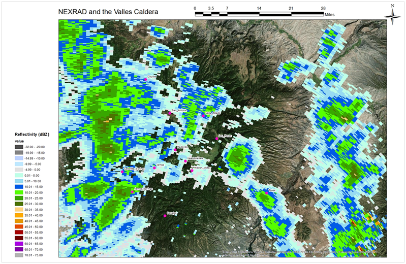
So, this means it’s snowing up there, right? (The data all come from January 5, 2016.)

Don’t be so quick to answer. Something was in the air that night, but daily gage readings showed zero or negligible snowfall.

The correlation between radar data and gage data is statistical at best. There are lots of factors affecting it. We’d love to come up with a best fit surface, and this will be the subject of my M.S. Thesis work.

For now, we continue to note the interesting features requiring our work. Let’s look at pixels.

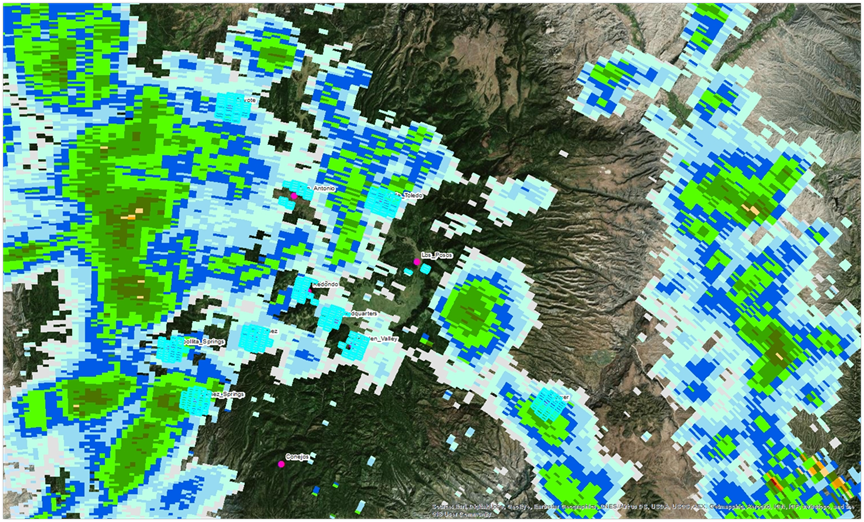
Above we see a single pixel of data (a few actually). At the distance of the Jemez, and single pixel is about .7 by .2 miles.

You could almost fit two distinct New Mexico thunderstorms into one pixel. Point data this is not!

The real crux of the question is how many pixels to use. On one hand, one pixel is way larger than a gage station.

But on the other hand, nearby pixels may have relevant information. Take a look.

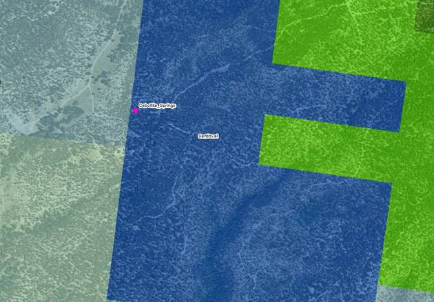
Cebollita Springs is in one pixel, a dark blue, but if the wind is at all from the west, the next pixel over is what really matters.

In fact, any number of surrounding pixels might matter. Perhaps we’ll want to select a bunch for analysis.

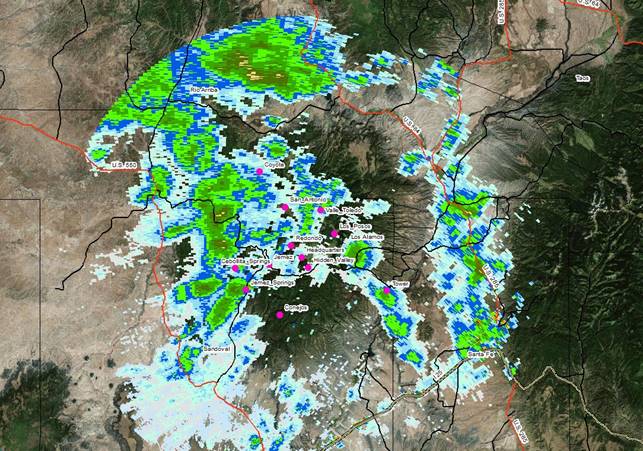
If we take all radar pixels within a mile of each station, we get this selection:

Some stations in the clear have no surrounding pixels to sample. Others are thoroughly surrounded.

Any analysis we do to get historic trends will have to account for nearby pixels, a size and distribution as yet to be decided, but ignoring the rest.

Of course, once the correlation function is determined, we use the remaining pixels to come up with a “best guess” about rain in any given point and time of interest.

Picking out this subset of pixels is not the only use for ArcGIS tools. We have a lot of data to work with, thirteen years-worth of gage stations and NEXRAD data.

At multiple elevation sweeps for but reflectivity and radial velocity (which we haven’t discussed here at all), doing five to ten an hour, that comes to perhaps 11 million files.

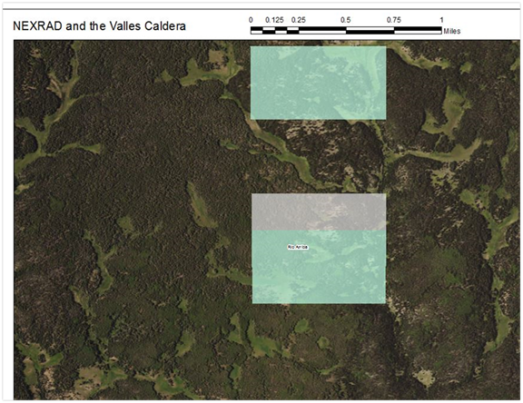
Let’s crop the raw data before we save and process it.

This picture is the end result of a multi-step process. I selected every pixel in a fifty mile range of headquarters.

Then I cut the rest out and saved this layer. We can reduce file sizes by at least 67% this way, as in this case.

With eleven million files to work through, this is important savings. Thank you ArcGIS!

Any and all interested parties may see how all this ends by attending my thesis defense, hopefully within 1 year from now (because I really want to graduate already).

Acknowledgements

Thanks to the National Park Service for sponsoring my work, of which the above is just an introductory slice.

Thanks to Mark Stone for being my advisor on said research.