Homework No. 3

Isabel Meza

Map Projections

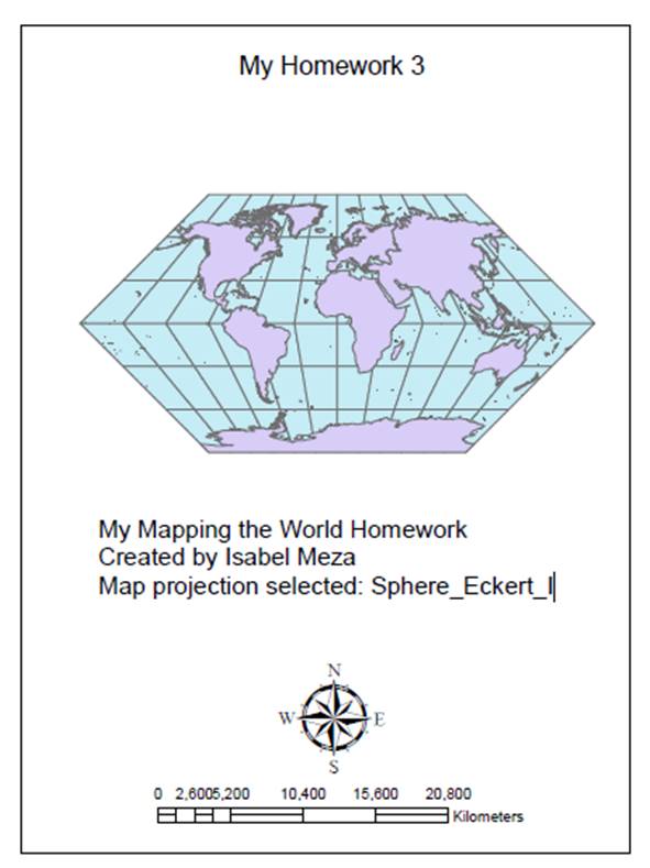
1) Mapping the World

For creating the first map, first, I opened ArcMap, and went to the right tab that shows Catalog. I created a new folder (geodatabase) in my own USB, so all the information and TempleData will be stored in that folder.

After I added all the layers that I was going to work in (World Continents and World Map background), I opened the Data Frame Properties, clicked under Coordinate System, and then I started playing with the different Projections found, until I found Sphere Ecker I and use it as my projection for this homework.

After that, I selected the Map Layout option and started inserting the legend, the title, and the basic information that I wanted to keep in my “Mapping the World Map”.

a. Provide a brief description of the projection and its parameters

I selected the Sphere Eckert I projection system, which is used primarily as a novelty map. It shows a pseudo cylindrical projection. Parallels and meridians are equally spaced straight lines. The poles and the central meridian are straight lines half as long as the equator. The parameters are: False Easting, False Northing, Central Meridian

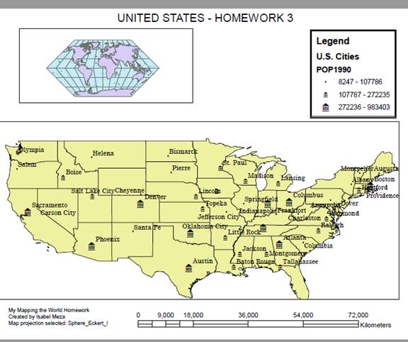
2) Mapping the United States

For the “Mapping the United States” map, I saved my first map, but started adding more layers in the same one, used for the first assignment question (no.1). I added the US. States and US. Cities from the TempleData which is already saved in my USB.

I clicked in the Layer properties, went to definition Query, and I clicked in the Query Builder button. I selected “Capital” under the Fields list, clicked =, clicked “get unique values” and selected the letter “Y”. Later on, I selected the “Verify Button, and then OK. It started showing me only the capital cities from the US. Later on I kept playing with it to see which cities were selected from the different options that I had, for example using “POP1990” and building the query with > 1,000,000, I could display all the cities which had population values higher than 1,000,000.

Later on, I started using the Symbology Tab, and started changing the symbols to be shown as the capital cities of my layer in “US CITIES”.

Later on, I clicked in the layer of the cities and selected the “label features” option. All the name of the cities appeared immediately.

I used the “magnifier” button, which is under the Windows Tab, in the main screen, and I could see an immediate “zoom in” of the place that I wanted to take a measurement from. I used the measure tool which is one of the buttons in the main screen (showing a ruler). Under the Date Frame properties, in the General tab, under the Display option, there are all the units that can be displayed in the map, using the “measuring tool”, so I changed the units and I could see the distances in different units. I did the same using a different coordinate system.

Later on, I started opening the Attribute table, and I started analyzing the different information found in it. The negative signs under the elevation column were showing a misted, because elevation usually is a positive number, so, when there is no elevation, then the number was showing -99. Answering the questions I found:

a. Determine the approximate latitude and longitude of three cities

-86.854832  36.109002 Decimal Degrees  Nashville-Davidson

-122.880317  47.039183 Decimal Degrees Olympia

-119.738987  39.137946 Decimal Degrees Carson City

b. What is the distance between Augusta and Olympia in miles if the view is not projected?

Under the projection that I had in the beginning, it was 2530.4 miles.

c. What is the distance between Augusta and Olympia in miles if the view is projected into Albers Equal Area? 2547.8 miles

d. In the Cities attribute table, why do think there are several values with –99 when looking into the elevation values? It represents a mistake, because that data does not exist or there was no elevation in this place.

e. What are the same distances in kilometers?

Without the projection: 4072,3 km and with the Albers Equal Area is 4100.3 km.

f. Which capital city is the most populous?

Phoenix, AZ with 983403 population density.

g. Which capital city is the least populous?

It is the city of Montpelier, VT with only 8247 population density.

h. Which capital city has the highest elevation?

I found that the city with the highest elevation is Santa Fe, NM 6989 feet above the sea level.

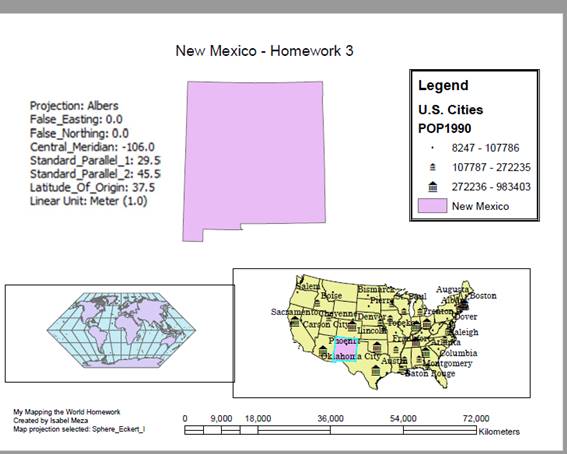
3) Mapping New Mexico a. List the projection parameters

For doing the New Mexico map, I selected the “select features” tool, and then I went to New Mexico and clicked on top of it.

Then clicking the States Layer, I selected export data, choosing the default geodatabase as the location of export.

I opened the ArcToolBox, went to Data Analysis Tools, clicked under Projections and found the projection that I wanted to work with.

I created a new Data Frame, under the name of New Mexico, added the projected polygon of the NM and when I was selecting the projection system that I was going to use, I clicked in Copy and Modify button, which was very complicated to find it, because in the assignment there was no explanation so ever to find that button, but after reading the Help information and the book, I could find it and I changed the value of the Central Meridian to -106.

Finally, I made out the layout look good, adding and moving the different data frames and got the last map:

This homework took a lot of time, because I couldn´t find the button or the way to change the Meridian information in the projection system properties.