NOTE: All layers must be projected and clipped to the watershed boundaries prior to use in AGWA. Prior to following the steps listed below the user must download AGWA, install the plug-in, and set the workspace folder.

Step 1: Watershed delineation and discretization

The user firsts performs a watershed delineation using a filled digital elevation model, flow accumulation, flow direction, and pour point. After the watershed is delineated it is subdivided into model elements.

Perform the watershed delineation by selecting AGWA Tools > Delineation Options > Delineate Watershed.

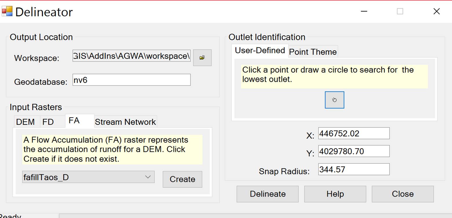
1.1. Output Location box:

1.1.1. Workspace textbox: navigate to and select/create C:\AGWA\workspace\CE_Final (This may need to be adjusted depending on where saved the downloaded AGWA file)

1.1.2. Geodatabase textbox: nv6 (This can be changed just assign a descriptive name to your geodatabase)

1.2. Input Grids box:

1.2.1. DEM tab: dem_Taos (this can be adjusted based on your site)

1.2.2. Press the Fill button. This fills the DEM, and creates the filldem_Taos raster.

1.2.3. FDG tab: Press the Create button. This creates the flow direction raster fdfill_Taos.

1.2.4. FACG tab: Press the Create button. This creates the flow accumulation raster fafill_Taos.

1.3. Outlet Identification box:

1.3.1. User Defined tab: (Choose a pour point location based on your Area of Interest.)

1.4. Click Delineate

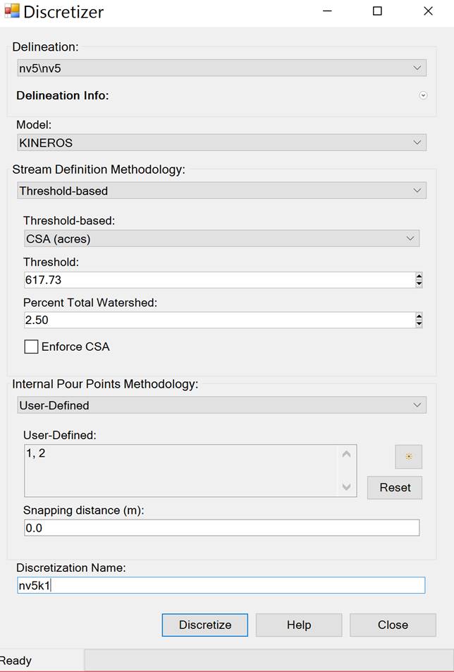
Step 2: Discretizing the Watershed

Perform the watershed discretization by selecting AGWA Tools > Discretization Options > Discretize Watershed.

2.1. Input box:

2.1.1. Delineation: nv5\nv5

2.2. Model Options box:

2.2.1. Model: KINEROS

2.3. Stream Definition box:

2.3.1. Method: CSA (Acres) 2.3.2. % Total Watershed: do nothing (it should read 2.5) 2.3.3. Threshold: do nothing (it should read 617.73)

2.4. Expand the Internal Pour Points box:

2.4.1. Select the User Defined tab page

2.4.2. Click yellow icon (select feature)

2.4.3. Select same location used for pour point in watershed delineation using flow accumulation grid

2.5. Output box:

2.5.1. Name: enter nv5k1( this is the name of your geodatabase and the KINEROS2 model number)

2.6. Click Discretize.

Step 3: Land cover and soils parameterization

AGWA requires inputs of both land cover and soil GIS coverages. During this step the watershed is intersected with these data and parameters necessary for hydrologic modeling are determined through a series of look up tables. The parameters are added to the polygon and stream channel tables.

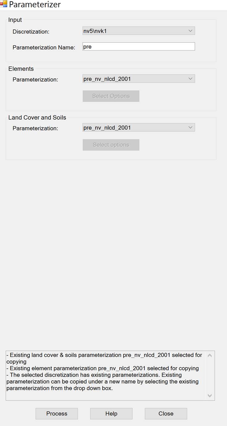
Perform the element, land cover, and soils parameterization of the watershed by selecting AGWA Tools > Parameterization Options > Parameterize.

3.1. Input box:

3.1.1. Discretization: nv5\nv5k1

3.1.2. Parameterization Name: pre

3.2. Elements box:

3.2.1. Parameterization: Create new parameterization

3.2.2. Click Select Options. The Element Parameterizer form opens.

3.3. In the Element Parameterizer form:

3.3.1. Flow Length Options: Geometric Abstraction

3.3.2. Hydraulic Geometry Options box:

3.3.2.1. Select the Eastern Arizona/New Mexico sites item.

Do not click the Recalculate button.

Do not click the Edit button.

3.3.3. Channel Type box:

3.3.3.1. Select the Natural item.

3.3.3.2. Click the Edit button.

3.3.3.3. Change the Hydraulic Conductivity to 0.

3.3.3.4. Do not change the Roughness and Armoring values.

3.3.4. Click Continue. You will be returned to the Parameterizer form to create the Land Cover and Soils parameterization.

3.4. Back in the Land Cover and Soils box of the Parameterizer form

3.4.1. Parameterization: Create new parameterization

3.4.2. Click Select Options. The Land Cover and Soils form opens.

3.5. In the Land Cover and Soils form:

3.5.1. Land Cover tab:

3.5.1.1. Land cover grid: nlcd_Taos (your NLCD layer in Arc Map)

3.5.1.2. Look-up table: mrlc2001_lut_fire

NOTE If the mrlc2001_lut_fire table is not present in the combobox, you may have forgotten to add the table to the map earlier. If this is the case, click on the Add Data button and browse to the C:\AGWA\datafiles\lc_luts\ folder and select mrlc2001_lut_fire, then select the mrlc2001_lut_fire table from the combobox.

3.5.2. Soils tab:

3.5.2.1. Soils layer: statsgo_Taos (the comp and layer files can be found in the AGWA datafiles\STATSGO\NewMexico it is easier if you join the tables based on the MUID during preprocessing)

3.6. Click Continue. You will be returned to the Parameterizer form where the Process button will now be enabled. Click Process

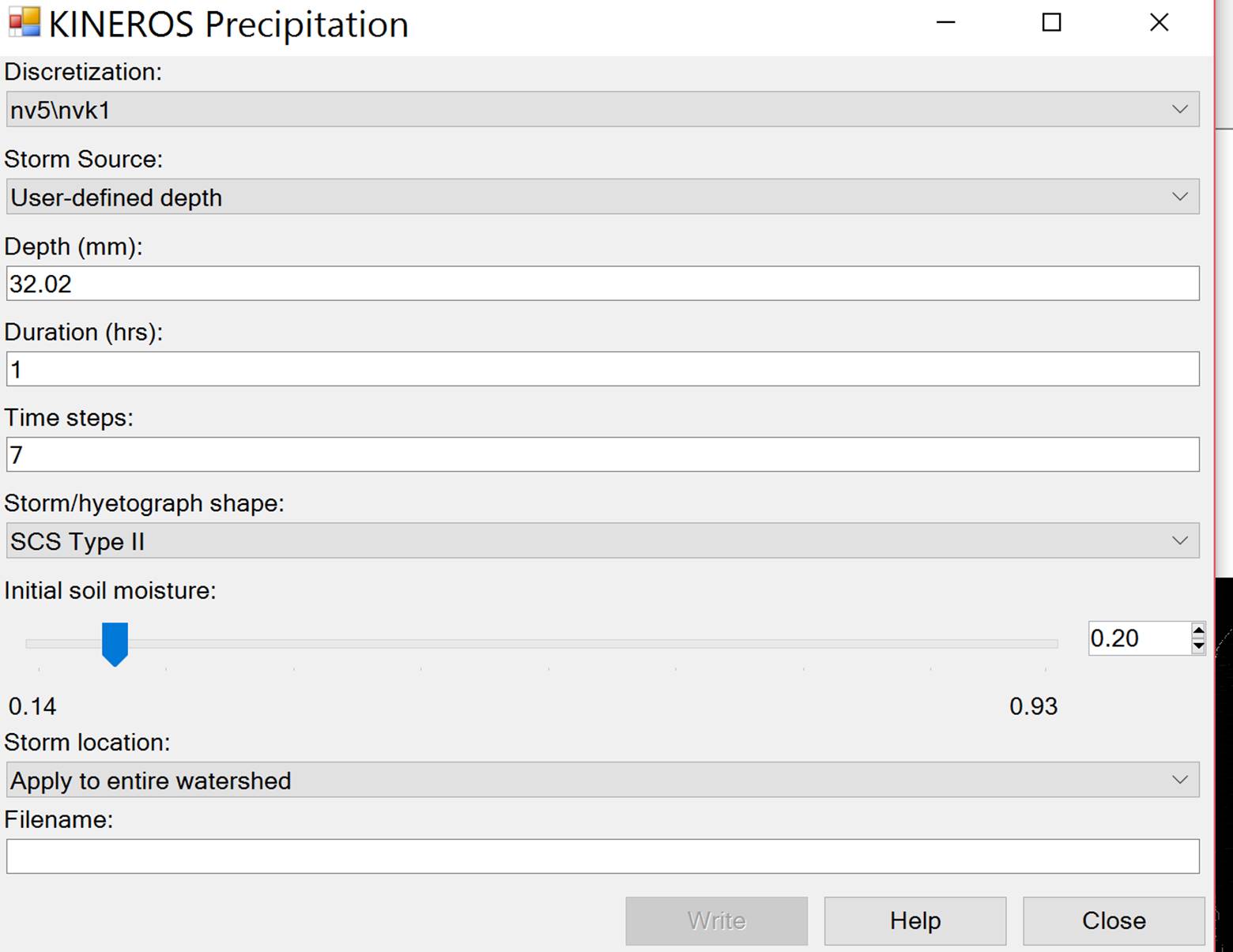
Step 4: Generating rainfall input files

4. Write the KINEROS2 precipitation file for the watershed by selecting AGWA Tools > Precipitation Options > Write KINEROS Precipitation.

4.1. KINEROS Precipitation form

4.1.1. Select discretization: nv5\nv5k1

4.1.2. Storm Depth box: 4.1.2.1. User-Defined Depth tab:

4.1.2.1.1. Time Steps: 7

4.1.2.1.2. Depth (mm): 32.02

4.1.2.1.3. Duration (hrs): 1

4.1.3. Storm Location box:

4.1.3.1. Select Apply to entire watershed radio button.

4.1.4. Storm/hyetograph shape: SCS Type II

4.1.5. Initial Soil Moisture: 0.20

4.1.6. Precipitation Filename: 10y1h

4.1.7. Click Write.

Step 5: Writing input files and running the model

Write the KINEROS2 simulation input files for the watershed by selecting AGWA Tools > Simulation Options > KINEROS Options > Write KINEROS Input Files.

5.1. Basic Info tab:

5.1.1. Select the discretization: nv5\nv5k1

5.1.2. Select the Parameterization: pre

5.1.3. Select the precipitation file: 10y1h.pre

5.1.4. Select the multiplier file: leave blank

5.1.5. Select a name for the simulation: 10y1hpre

5.2. Click Write.

Step 6: Executing the model

6. Run the KINEROS2 model for the Andreas Canyon watershed by selecting AGWA Tools > Simulation Options > KINEROS Options > Execute KINEROS Model.

6.1. Select the discretization: d1\d1k1

6.2. Select the simulation: 10y1hpre

6.3. Click Run. The command window will stay open so that successful completion can be verified. Press any key to continue. Close the Run KINEROS window. (NOTE: The AGWA Run KINEROS window in arc map will not close if you do not close the Windows Run Command Window)

Step 7: Creating Post-Fire Land Cover

Perform the land cover modification for the post-fire land cover by selecting AGWA Tools > Other Options > Burn Severity Tool.

7.1. Inputs box:

7.1.1. Burn severity map: TAOS_SBS (This layer must be created using a burn severity raster map/clipping to the burn boundary/converted to a polygon using the “raster to polygon” tool is arc toolbox/ Then use “Dissolve” to merge based on burn severity class (1-4)/ lastly you must use the editor tool in arc map and add the total number of acres in each burn severity class.)

7.1.2. Severity field: GRIDCODE

7.1.3. “Low” severity index: 2

7.1.4. Land cover grid: nlcd_Taos

7.1.5. Change table: mrlc2001_severity

7.2. Outputs box:

7.2.1. Output folder: navigate to and select C:\AGWA\workspace\tutorial_MountainFire\ 7.2.2. New land cover name: postfire

7.3. Click Process.

Step 8: Reclassify Post Fire NLCD

8. At this point, the postfire raster representing the post-fire land cover has been created. To better visualize the different land cover types and associate the pixels with their classification, load a legend into the nlcd_Taos and postfire datasets.

8.1. To do this, right click the layer name of the nlcd_Taos dataset in the Table of Contents and select Properties from the context menu that appears.

8.2. Select the Symbology tab from the form that opens. In the Show box on the left side of the form, select Unique Values and click the Browse button on the right. Click the file browser button, navigate to and select C:\AGWA\datafiles\renderers\nlcd2001.lyr and click on Add, then click OK to apply the symbology and exit the Import Symbology form.

8.3. Click on Apply in the Layer Properties form and then on OK to exit this form.

8.4. The nlcd_Taos and postfire datasets have the same legend and classification, so repeat the same procedure for the postfire dataset.

REPEAT STEPS 2-5 WITH THE POST FIRE LAND COVER