


Background
The former Division of Government Research (DGR) at UNM developed a special purpose gravity model for measuring geographic access to health care facilities and providers in New Mexico. This work was performed for the former New Mexico Health Policy Commission (NM HPC) from 1988 through 2002. The results of this preliminary work were only published on DGR's former web page and also in a limited distribution publication by the NM HPC ( HPC Quick Facts 2003 - color extract). A special poster presentation was also prepared that won the poster contest at the 2002 ESRI SWUG Conference held in Taos, New Mexico ( now Esri Southwest User Conference).
The gravity model was very innovative and potentially useful in many other places beyond New Mexico where having a higher resolution, more accurate and reliable measure of geographic accessibility to health care would benefit policy decisions. This research will continue the development of this gravity model (see the Story Map) and also compare it with results obtained from recently developed techniques used by other researchers. The original gravity model was developed using (SAS) and ESRI's ArcGIS. These updates will be done using ArcGIS ModelBuilder, Python scripts, R, and now with ArcGIS Pro.
Note: Most of the effort so far has concentrated on technical development, learning and applying various computing programming and statistical software facilities. The resulting models and scripts will eventually be made available for other researchers to use and modify. Hopefully these technical developments will clearly demonstrate the use of this improving GIS technology and encourage state agencies to resolve data quality and data sharing issues. Esri has also been encouraging government agencies to participate in their Open Data program which hopefully may result in more New Mexico data becoming available for public use in the future. For more recent official information about the status of New Mexico's health care workforce please see New Mexico Health Care Workforce Committee Annual Reports. Also see Modeling Future Health Care Workforce Adequacy to Inform Policy.
Initial Updates (2012 to 2015)
I recently made progress developing an ArcGIS ModelBuilder version of this gravity model using ZIP Codes and older provider data (previously available). For now, there is a map (PDF) of the preliminary results of Population per Primary Care Physician plus a (PDF) showing the design and components used for ArcGIS ModelBuilder available below. Most recently, I have begun the process of developing a Python script tool and there is documentation with screen shots available below that will be updated as this process continues (also see the class presentation). Currently, the Python script tool works well except that I am having problems fully automating the symbology with user defined input for the class breaks. For now, the last step is a manual process where symbology can be modified from the default natural breaks classification. I hope to resolve this problem with ESRI technical support in the future.
The results still need to be verified for accuracy by comparing them to those obtained using the existing SAS Macro developed at DGR. However, I no longer have access to a Windows version of SAS as I had for many years as a UNM staff employee. At UNM there is no student version of SAS available for installation on personal computers like at many other universities such as PSU, BU, Texas A&M, and Stanford. The Windows version is only available for student use in a few computer pods and for departmental use purchased with a UNM account. There is a Linux version, but disk space quotas limit its utility. SAS recently relased a new University Edition that will allow comparision, but it lacks the SAS Bridge that works with the Windows version that would be very helpful. I still hope to use the SAS Bridge in combination with ArcGIS ModelBuilder and Python scripts (add-ins). I'm not sure yet which will prove to be more efficient. I still intend to make the ArcGIS ModelBuilder and Python scripts available sometime in the future once properly documented and packaged for others to use.
I still plan some more developments using census tracts and geographic units other than ZIP Codes such as the New Mexico Small Areas developed by the New Mexico Department of Health (see the Story Map - first version). Hopefully, geocoded provider and facility data can be obtained in the future that would allow comparision of results with other established techniques such as IDW, Kernel Density and the two-step floating catchment area method (2SFCA). Also obtaining recent provider and facility data for the border areas of states adjacent to New Mexico (Arizona, Colorado, and Texas) would provide more reliable results as many patients cross the state boundary and some also go to Mexico for care. The boundary/edge problem is a very common methodological problem that should be addressed in the proper design of spatial analysis applications. Further, if a good New Mexico road network database were developed for use in the ArcGIS Network Analyst , actual travel distance and time on the roads can be used instead of Euclidean distances. It would be interesting to compare results and see if any major improvements become apparent given the effort involved in creating a good road network dataset for the state. However, this effort is sorely needed for many other network based applications beyond just those for healthcare.
Given some minor problems that still need to be resolved with ArcGIS (mostly automating symbology) I have begun exploring using QGIS and Python for the health care gravity model. A general Python version of the gravity model is currently being developed that will allow for the use of both ZIP Codes, census tracts, and the New Mexico (NMDOH) Small Areas for any type of health care providers and facilities. I hope to have versions that that will work in both ArcGIS and QGIS. I will post results as I become more familiar with this open source GIS in the future.
I have also tested a revised version of the SAS gravity model using census tracts and the New Mexico (NMDOH) Small Areas with 2002 population estimates and 2002 primary care physician data (see Small Area Map and Census Tract Map). Note: A spatial join was used to assign ZIP Code physician data to census tracts and NMDOH small area. In the future, geocoded physician locations would be more accurate. However, given the interpolation performed by the gravity model I think the results would not be very different. Some of these results will be available on ArcGIS Online in several GIS formats (interactive web maps, map package, map services, map layers, and shapefiles) as development continues. I was recently provided with an organizational account when I renewed my home use license for ArcGIS which I never had before. Thanks esri!
I have prepared a Python (GDAL/OGR) script that reads a shapefile, calculates the gravity model, and writes a new shapefile with original data and results. I have mostly finished converting this python script into a QGIS processing script to allow for more user interaction and eventually automated display of results (see screenshot of curently working user interface and documentation). I may also consider the option of preparing a QGIS graphic modeler once the QGIS processing script is completed. I have also begun developing a QGIS plugin (see documentation) based on these scripts that will be made available for public use (see the QGIS Plugin Repository). The shared plugin will be generic (could be used in places other than New Mexico). For now only a screenshot of the results from QGIS are available until the plugin is completed. In addition, more developments using Ubuntu-Linux and other open source geospatial software are planned for the future. Note: Although QGIS developments are being prepared using Ubuntu-Linux they will also work on the Windows and Mac versions (see screenshot of the Windows processing script user interface). Links below with these developments will be posted soon!.
As I now have working Python code QGIS(PyQGIS) for the DGR gravity model I have also developed a mostly Python script (see documentation) using ArcGIS(ArcPy) and have started developing a R function. My earlier development of an ArcGIS ModelBuilder application and Python script tool derived from ModelBuilder proved too cumbersome and slow although it worked well. As both ArcGIS (R-ArcGIS) and QGIS (external application) have developed improved interfaces for R, now is a good time to do some more development with this widely used open source statistical software.
New Developments (Ongoing since 2015)
- I have begun exploring the infogroup data recently obtained by the NM Department of Information Technology and provided by the NM Community Data Collaborative as a source for more up-to-date healthcare data for use with the DGR gravity model. The preliminary results (see ArcGIS Online Web Map) using unedited data are promising. I will be using both UNM's GPS and Esri Demographics as the source for population data estimates at the census tract and also the block group levels of geography. There some differences at the census tract level between both of these estimates (see ArcGIS Online Web Map Viewer - NM 2015 Census Tract Population Estimates) and only Esri provides estimates for block groups. I will also be using SAS to prepare the data for subsequent use and resolve data quality issues. Further work is necessary to compare this data with state licensing databases and other sources such as the US News Doctors Listings. This will help to verify active providers and workloads plus removing multiple data entries and duplicate records. The gravity model will become more useful as the quality of the data gradually improves.
- As Esri continues to improve the integration of ArcGIS with open source statistical packages (see 2016 Developer Summit Tech Session), I am developing an updated Python script using the Spatial Statistics Data Object. I have also begun to use the R-ArcGIS Bridge for both accessing ArcGIS from R Studio and also to develop an R Script Tool in ArcGIS Pro (see ArcGIS Blog and 2016 Developer Summit Tech Session). An R Script that uses a spatial data frame was completed as part of a class I recently finished (Geog 580L - Spatial Statistics - Spring 2017). The DGR gravity model results were also compared to selected socio-economic factors using Geographically Weighted Regression (GWR). A PowerPoint presentation describing these exploratory results is available.
- Based on previous developments, I have started to prepare an R function for the DGR gravity model. I also intend to prepare a R script version of the (2SFCA) gravity model and compare results with the earlier gravity model developed by DGR. These developments should be available in the future after more development and testing.
- I am continuing to expand my efforts in this area and more developments are planned. The main purpose and research goal is to compare various geographic access and gravity models (DGR, 2SFCA, and E2SFCA) at more detailed levels of geography than New Mexico counties (by census tract and perhaps ZIP Code). Although it would be helpful if up-to-date provider data maintained by UNM Health Sciences were eventually available, other cuuuently available and less accurate data sources can be substituted for testing. There are currently available population estimates provided by Esri and also UNM Geospatial and Population Studies (GPS). As part of this work I intend to use both aggregated (by census tract) and geocoded provider data. Also, both Euclidean and road network (distances and travel times) measurements will be evaluated. Additional research could be conducted to analyze various socio-economic factors (Census ACS and Esri's Tapestry-Lifestyle data) and selected health indicators (NM DOH - IBIS) to evaluate relationships with various geographic accessibility model results using several spatial regression methods. Both R and Python in combination with ArcGIS Pro will be used for this work and Esri's recent technical developments should prove helpful. Results will be posted here as progress is made.
- Previously: (for Geog 591 - Problems - Fall 2017)
focused on ArcGIS Pro Python script tool developments
for the various geographic access and gravity models (DGR,
2SFCA,
and E2SFCA)
with additional Python libraries (Pandas,
SciPy,
NumPy,
and GeoPandas).
I am learning Anaconda,
Jupyter Notebooks,
and PyCharm.
Both Euclidean distances (Numpy Arrays) and road based distances (
ArcGIS Pro OD Cost Matrix)
will be used for statistical comparisons.
A test case using only the 33 New Mexico counties
and a selected populated place (county seat or other city-town) has been prepared.
This development test used more reliable 2015 physician data
prepared by UNM Health Sciences
and population estimates from UNM's GPS at the county level.
These results are promising (see Euclidean Distance Map,
Road Distance Map,
Web Map or
Web Map Application).
Gravity model measures of potential geographic accessibility that remove the effects of political (county) or
other data collection (census tracts, zip codes, etc.) boundaries creates a more complete and realistic picture as patients freely
move across boundaries to obtain healthcare services. The traditional county based (service capacity standard) methods provide
only a partial measure of accessibility.
The county based test case results can be further modified to disregard county boundaries using the
ArcGIS Inverse Distancw Weighted Tool (see IDW - Road Distance Map),
but this smoother statistical surface should be interpreted with more caution.
I have derived an OD Cost Matrix for all of the New Mexico census tracts using the Origin Destination Cost Matrix Tool. The DGR gravity model can now be applied with road based distances. For now, I will use the 2002 primary care physician data that was previously available during the earlier work performed by DGR for the New Mexico Health Policy Commission (NM HPC) from 1988 through 2002. Although this previous work was based on ZIP Codes, recent adjustments ( spatial join) have been performed (see the Story Map) to use census tracts and 2002 population estimates from UNM GPS. These results are very informative (see 2002 Gravity Model - Road Distance Map). The census tract test case results can be further modified to disregard county boundaries using the ArcGIS Inverse Distancw Weighted Tool (see IDW - Road Distance Map), but this smoother statistical surface should be interpreted with more caution. A Web Map and Web Map Application). are also available with these results. If the recent physician data for census tracts (499) or ZIP Codes (426) are eventually made available, the DGR gravity model results can provide a higher resolution and more useful picture of geographic accessibility.
Begun to focus on the primary research goal, to statistically compare various geographic access and gravity models (DGR, 2SFCA, and E2SFCA) at various levels of geography including those with higher resolution than New Mexico counties (by census tract, ZIP Code, and perhaps census block group). Also to compare the results for each model using both Euclidean and road based distances. Preliminary results have been informative and somewhat suprising. There are pronounced differences ( measured using both relative difference and correlation coefficent) between the results when comparing Euclidean and road distances for the DGR gravity model at the county (r = 0.8088695) and census tract (r = 0.6584075) levels of geography (see 2015 County Relative Difference Map or 2002 Census Tract Relative Difference Map or Web Map or Web Map Application). Obviously accessibility depends on where you are located with respect to the network of roads. Assumming equal accessibility as measured by Euclidean distance (isotrophic surface) is not very realistic. The geography of New Mexico supports this, although I did not think the differences woud be as large as they are in some places.
- Note: Based on a review of published research (see Wang, 2017) I have decided to refer to the DGR gravity model as the "One-Step Hybrid Gravity Model" (1SHGM) method. This earlier work was influenced by classical retail oriented gravity models and designed at the time to fit the special circumstances of New Mexico.
-
Recently: (for Geog 528 - Advanced Programming for GIS - Spring 2018)
Continuing the focus on the primary research goal, to statistically compare various geographic
access and gravity models (1SHGM,
2SFCA, and E2SFCA)
at various levels of geography including those with higher resolution than New Mexico counties
(by census tract, ZIP Code, and perhaps census block group).
Also to compare the results for each model using both Euclidean and road based distances.
In order to check the results additional developments will be performed for various models using
both the
SAS University Edition
, Python - GeoPandas
and perhaps QGIS(PyQGIS).
I have started using the Two-Step Floating Catchment Area (2SFCA) methods with the ArcGIS Desktop (ArcPy) script tools provided by Dr. Fahui Wang ( Wang, 2017). A Web Map showing results for the generalized 2SFCA method has been prepared using the 2002 primary care physician data that was previously available during the earlier work performed by DGR for the New Mexico Health Policy Commission (NM HPC) from 1988 through 2002. This class provided an excellent review and more in-depth background for various Python modules including Python - GeoPandas. I have re-programmed the generalized two-step floating catchment area methods using both SAS and Python3 - GeoPandas within Jupyter Notebook (see class PowerPoint Presentation). However, I did not make as much progress as I would have liked on the statistical comparison portion of my research project and more work will continue this summer and during the fall semester.
 Recently: (Summer 2018 and for Geog 591 - Problems - Fall 2018)
Continuing the focus on the primary research goal to statistically compare various geographic
access and gravity models (1SHGM, 2SFCA, and E2SFCA).
Some minor modifications of the previously developed
Python3 - GeoPandas
code are necessary and still need to be completed
to allow for a better comparision to the DGR-1SHGM method
that follows the specifications set out by the New Mexico State Legislature
(Senate Joint Memorial 36, 1996) that suggests maximum travel time of 45 minutes or about 35 miles of distance
(rule based, three-zone hybrid approach).
Also more work needs to be done to combine the various methods (1SHGM, 2SFCA and E2SFCA) with
a better user interface and flow of control using the
PyCharm IDE.
This modified code is currently being prepared plus
a detailed statistical comparison of these results using the
SAS University Edition
and the R-ArcGIS Bridge
will be available as progress is made.
In addition, the spatial access ratio (SPAR),
a recently developed method used to reduce uncertainty in model results has been employed by other researchers
(see
recent publication by a UNM research group).
I plan to compare the SPAR with both the one-step and two-step model results as part of future analyses.
I am also working on developing a version using the new
ArcGIS API for Python
and have been able to perform the calculations using the
SpatialDataFrame
but have not been able to directly display the results (see
GeoNet Question).
I have also started to develop another version using both NumPy and Pandas in
ArcGIS Pro
with
FeatureClassToNumPyArray (see
Python: Working with Feature Data) but there is not yet a direct way to go back to a feature class
from a Pandas data frame (see GeoNet Question).
Eventually, there will be a Story Map with a discussion and results.
Recently: (Summer 2018 and for Geog 591 - Problems - Fall 2018)
Continuing the focus on the primary research goal to statistically compare various geographic
access and gravity models (1SHGM, 2SFCA, and E2SFCA).
Some minor modifications of the previously developed
Python3 - GeoPandas
code are necessary and still need to be completed
to allow for a better comparision to the DGR-1SHGM method
that follows the specifications set out by the New Mexico State Legislature
(Senate Joint Memorial 36, 1996) that suggests maximum travel time of 45 minutes or about 35 miles of distance
(rule based, three-zone hybrid approach).
Also more work needs to be done to combine the various methods (1SHGM, 2SFCA and E2SFCA) with
a better user interface and flow of control using the
PyCharm IDE.
This modified code is currently being prepared plus
a detailed statistical comparison of these results using the
SAS University Edition
and the R-ArcGIS Bridge
will be available as progress is made.
In addition, the spatial access ratio (SPAR),
a recently developed method used to reduce uncertainty in model results has been employed by other researchers
(see
recent publication by a UNM research group).
I plan to compare the SPAR with both the one-step and two-step model results as part of future analyses.
I am also working on developing a version using the new
ArcGIS API for Python
and have been able to perform the calculations using the
SpatialDataFrame
but have not been able to directly display the results (see
GeoNet Question).
I have also started to develop another version using both NumPy and Pandas in
ArcGIS Pro
with
FeatureClassToNumPyArray (see
Python: Working with Feature Data) but there is not yet a direct way to go back to a feature class
from a Pandas data frame (see GeoNet Question).
Eventually, there will be a Story Map with a discussion and results.
Exploratory Data Analysis: Some very preliminary results and data visualizations are now available that have been prepared using the SAS University Edition. These results (see summary statistics PDF) suggest that there is a significant difference in the results obtained from the 2SFCA methods compared with the 1SHGM method. However, these results based on a standard ANOVA should be interpreted with caution as several of the basic ANOVA assumptions are not met, primarily the independence of the data that are spatially autocorrelated and also not normally distributed plus non-common variances. More work is currently underway to research and apply more appropriate statistical methods. These additional statistical methods within R will be used to compare results from various models (one-step vs. two-step with various distance decay functions) and will be available as progress is made (see R Results). In addition, both absolute and relative differences will be calculated to investigate how results vary at each census tract location (see Preliminary Results (1SHGM and 2SFCA) Web Mapping Application - Note: a more efficient version is being prepared using the ArcGIS API for JavaScript).
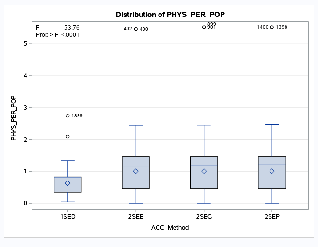
Hybrid-Zonal Model Results with Various Distance Decay Functions: The boxplot (below) shows the distribution of Physicians per Population (PHYS_PER_POP) from the various models (Acc Methods - Accessibility Methods), all using a hybrid-zonal approach with various distance decay functions (1SED - 1SHGM with DGR type power distance decay; 2SEE - 2SFCA with exponential distance decay; 2SEG - 2SFCA with gaussian distance decay; 2SEP - 2SFCA with power distance decay). Note: the means and medians are close for the 2SFCA and only slightly different than the 1SHGM. It may be that the ANOVA results (can reject the null hypothesis that the means of the different methods are the same p < 0.0001 and accept the alternative hypothesis that at least one mean is not equal to the others) have been greatly influenced by the different variances and presence of extreme outliers.
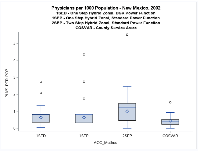
Power Based Distance Decay Results: This boxplot (below) and histograms and boxplot PDF. shows the distribution of Physicians per Population (PHYS_PER_POP) from various models (Acc Methods - Accessibility Methods), using a hybrid-zonal approach with power based distance decay functions and also the distribution using the county based service area approach (COSVAR). This visual comparison indicates that the one-step methods (1SED and 1SEP) tend to produce more similar results to the widely used county based service area method (COSVAR) than a reasonably comparable two-step method (2SEP). An interactive web map has been prepared showing these results and the relative difference between the one-step and two-step methods at each census tract. There are also some special web mapping applications (see 1SEP and 2SEP, 1SED and 2SEP, and 1SED and 1SEP) that are more useful for comparing these results side-by-side. Note: The county based service area method (COSVAR) is only a population-to-physician ratio, it's the service capacity standard or "rational service area" used by the U.S. Department of Health and Human Services (DHHS) for defining physician shortage areas.
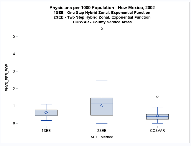
Exponential Distance Decay Results: This boxplot (below) and histograms and boxplot PDF. shows the distribution of Physicians per Population (PHYS_PER_POP) from various models (Acc Methods - Accessibility Methods), using a hybrid-zonal approach with exponential based distance decay functions and also the distribution using the county based service area approach (COSVAR). This visual comparison indicates that the one-step method (1SEE) tends to produce more similar results to the widely used county based service area method (COSVAR) than a reasonably comparable two-step method (2SEE). An interactive web map has been prepared showing these results and the relative difference between the one-step and two-step methods at each census tract. There is also a web mapping application that is more useful for comparing these results side-by-side. Note: The county based service area method (COSVAR) is only a population-to-physician ratio, it's the service capacity standard or "rational service area" used by the U.S. Department of Health and Human Services (DHHS) for defining physician shortage areas.
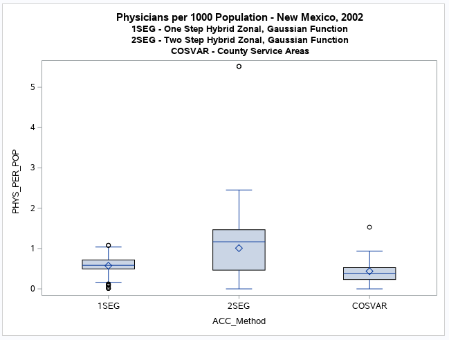
Gaussian Distance Decay Results: This boxplot (below) and histograms and boxplot PDF. shows the distribution of Physicians per Population (PHYS_PER_POP) from various models (Acc Methods - Accessibility Methods), using a hybrid-zonal approach with Gaussian based distance decay functions and also the distribution using the county based service area approach (COSVAR). This visual comparison indicates that the one-step method (1SEG) tends to produce more similar results to the widely used county based service area method (COSVAR) than a reasonably comparable two-step method (2SEG). An interactive web map has been prepared showing these results and the relative difference between the one-step and two-step methods at each census tract. There is also a web mapping application that is more useful for comparing these results side-by-side. Note: The county based service area method (COSVAR) is only a population-to-physician ratio, it's the service capacity standard or "rational service area" used by the U.S. Department of Health and Human Services (DHHS) for defining physician shortage areas.
Summary of Results: My initial goal for this research project was to compare the one-step and two-step models given an assumption or hypothesis that there would not be any significant differences as both are essentially gravity models. However, I have been surprised by the results. There is clear evidence of a significant difference between the one-step and two-step models that have similar constructs (hybrid-zonal) and employ the same distance decay methods (power, exponential, or Gaussian).
It is important to note that there is no indication that either model is a better measure of reality than the other. This can perhaps only be determined when actual observational provider data records are reviewed, or statistical patient-based surveys are conducted . As these models are only approximations of reality, a given model can only be evaluated as somewhat more appropriate or suitable than the other given the availability and quality of input data, plus how well it matches the desired usage or purpose.
This project has been an exceptional learning exercise that has enabled me to gain a better understanding of statistical, spatial, and GIS software and techniques. I have focused on presenting the results as objectively as possible. However, I do have some personal observations that are worth presenting for discussion purposes. Hopefully other researchers will review these results and make future suggestions that will aid in my interpretations.
The one-step models are easier to operationalize but conceptually provide lower resolution than the two-step models. They can require using less computational resources and GIS facilities. However, it is necessary to calculate road-based distances and use a GIS to display results on a map. Also standard statistical packages and programming environments can be used to perform most of the calculations. The results seem to be more similar to the traditional county-based service capacity standards used by the federal government for measuring physician shortage areas. The mean values are similar to the statewide means and have smaller variances. Although they appear to spread out the potential accessibility measures more evenly, they can also over-estimate in actual shortage areas. Regardless, the one-step model may be a good initial first step beyond the traditional county-based methods. They are easier to explain to decision makers such as state legislators as they are a simple extension of the standard service capacity ratio measure. A one-step model may be more suitable at the state level of geography than a similarly constructed two-step model. As such, it may be a more appropriate choice for healthcare planners seeking necessary increased funding.
The two-step models require more effort to operationalize but conceptually provides higher resolution than the one-step models. More computational resources and GIS facilities are required. A more involved programming effort within the GIS and related scripting environments is necessary as the calculations are more complicated. The resulting mean values are noticeably larger and variances greater than the traditional county-based service capacity standards used by the federal government for measuring physician shortage areas. They seem to not spread out potential accessibility measures as evenly as the one-step models and may perhaps over-estimate and severely under-estimate in some areas. Regardless, they represent a definite technological advancement that should be applied when appropriate. However, they are more difficult to explain to a non-professional audience. A two-step model may be more suitable at the urban and regional levels of geography than a similarly constructed one-step model. Several varieties of two-step models are continuing to be developed by academic researchers and their parctical applications have been demonstrated.
There is more research work to be undertaken in evaluating the similarities and differences (comparing and contrasting) between the one-step and two-step models. This study used the ZIP-Code (post office locations or centroids) to locate physicians because this older data was all that was available. More recent physician data, if available, could be used to more accurately geocode addresses. From a more technical perspective, the effects of both the modifiable areal unit problem (MAUP) and mathematical aspects of the calculations need more evaluation. It is also apparent that healthcare planners could benefit if better scripting applications were developed. These developments could make it easier to review results and allow for better selection of an appropriate model to employ.
-
Recently: (for Geog 591 - Problems - Spring 2019 and Summer 2019)
I have started working on completing a more in-depth statistical analysis and review of the one-step and two-step models.
These more detailed results will eventually be presented using Esri's ArcGIS Online
Story Map facility.
I am also evaluating several ways to develop improved scripts using
Python3 - GeoPandas
and the PyCharm IDE.
A QGIS(PyQGIS) script, plugin, and standalone application
will eventually be developed providing GeoPandas is compatible with the new QGIS 3.x versions.
Given recent developments in
the ArcGIS API for Python
and the new
Spatially Enabled DataFrame (SEDF)
this may now provide an efficient web based development environment.
The SEDF can now be used within
ArcGIS Pro (ArcPy) and I will also explore developing a jupyter notebook and script here
using a special Conda environment.
Eventually these Python scripts (see draft documentation)
will calculate selected models, compares results using both exploratory and statistical data analysis methods,
plus hopefully include a spatial version of ANOVA.
Note: please see
"All models are wrong but some are useful".
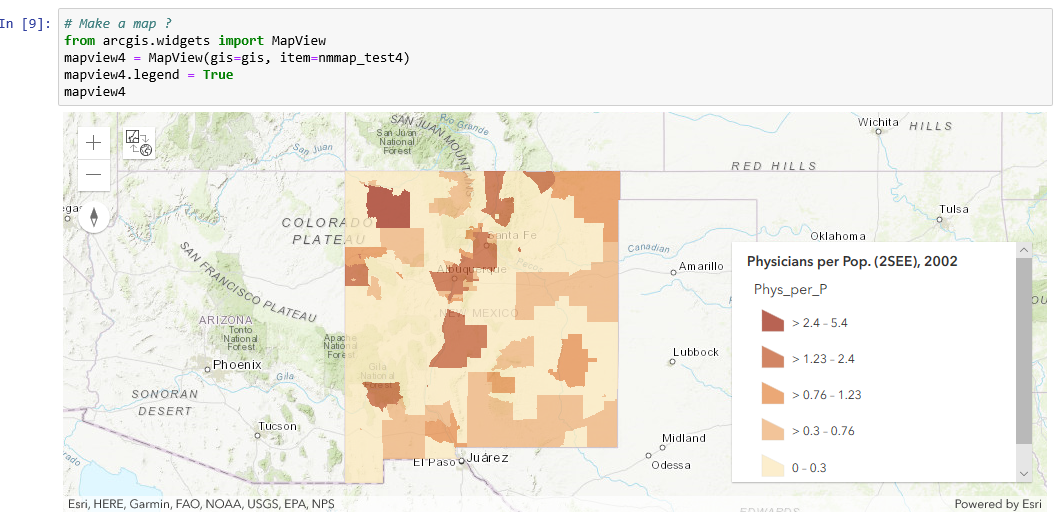
I spent more time than expected this summer viewing selected technical sessions from the recent Esri Developer Summit and becoming familiar with the ArcGIS API for Python and the new Spatially Enabled DataFrame (SEDF). Replacing GeoPandas with the SEDF was easy and the calculations of a test 2SEE model were successful. However, the map visualization of results within Jupyter Notebook was more problematic. Using an ArcGIS Online WebMap with the Jupyter Notebook Mapping Widget (arcgis.widgets.MapView) was the best alternative as it allows for a map legend to also be displayed (see below). But I have had problems after adding a results layer directly to the webmap. I can't display the polygon symnology without saving it to ArcGIS Online for rendering with smart mapping and then loading it again in another jupyter notebook cell to display. I hope to learn more about the proper way to do this and resolve my problems shortly.
-
Recently: (for Geog 591 - Problems - Fall 2019)
I am still working on completing a more in-depth statistical analysis and review of the one-step and two-step models.
These more detailed results will eventually be presented using Esri's ArcGIS Online
StoryMap facility.
I hope to make more progress evaluating several ways to develop improved scripts using
Python3 - GeoPandas
and the PyCharm IDE.
A QGIS(PyQGIS) script, plugin, and standalone application
will be developed providing GeoPandas is compatible with the new
QGIS 3.x versions.
However, I think
ArcGIS Pro is currently the most suitable GIS environment for development given the new
ArcGIS API for Python and the
Spatially Enabled DataFrame (SEDF).
I will also be using the Spyder IDE for developing a
geoprocessing script tool.
I will continue more research to see if a spatial version of ANOVA can be included with the
exploratory and statistical data analysis methods used in these scripts to compare results and
allow the user to make a more informed decision of which model to use.
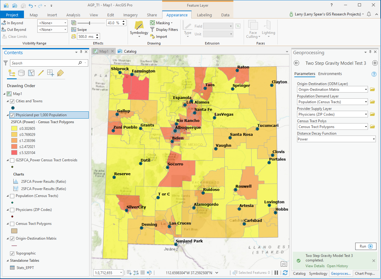
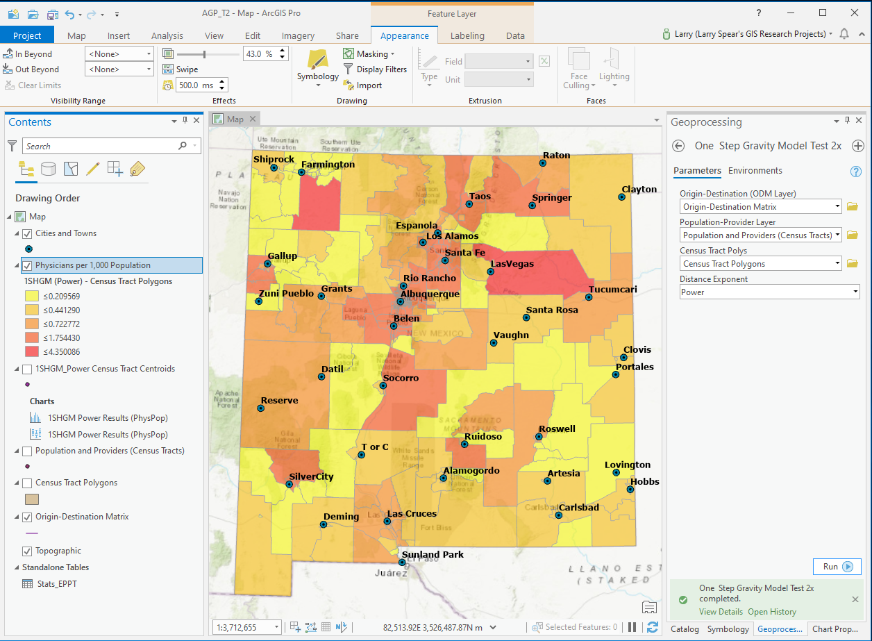
I have been making good progress developing a geoprocessing script tool for both the 1SHGM and G2SFCA
models (exponential, Gaussian, powers including DGR's variation) using ArcGIS Pro and the API for Python
that also includes diagnostics such as summary statistics, histogram, and a boxplot (see preliminary test versions
below).
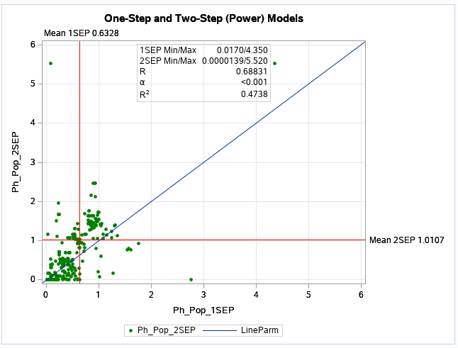
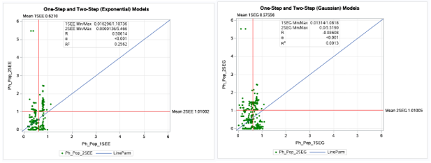
Although the model results and maps (natural breaks) are similar in many census tracts, there are
noticeable differences in the physician per population values for other census tracts
that influence the statistical comparisons (see scatter plot below).
Additional statistical comparisons of results plus
technical documentation for these geoprocessing tools are currently being prepared and will be available soon.
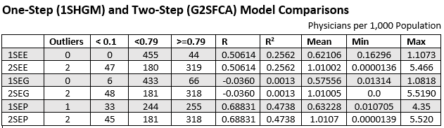
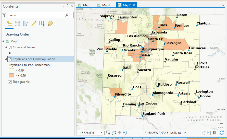
The additional statistical analyses of results has clearly shown that significant differences are apparent in the comparisons of the one-step (1SHGM) and two-step (G2SFCA) models. A series of scatterplots were prepared and correlation coefficients were calculated that support the results obtained from the previous histograms and T-Tests. The table (see below) summarizes these results. The most similar results when comparing the one-step and two-step models was for those that used a power based distance decay method (1SEP and 2SEP). The one-step (1SEP) model also seemed to produce the most realistic results with a mean value close to the statewide mean (0.6225) and a more even numerical distribution of census tracts below (244) and at or above (255) the national proviter-to-population benchmark (0.79). However, there was not a very even geographical distribution (see map below) as most of the census tracts below the benchmark seem to be in the larger rural census tracts with some exceptions in the southern and southeastern urban areas close to New Mexico's borders with Arizona, Texas and Mexico. Additional research using spatial statistical regression models is planned that will evaluate how results from these geographic access models are related to various measures of health inequality and health disparities.
-
Currently: (Independent Research 2020 - 2022)
I am continuing work to develop both a QGIS
and ArcGIS Pro
geoprocessing scripts for the one-step and two-step models.
I will also be using both Conda
Python and R enviornments
with Jupyter Notebooks and the new
ArcGIS Pro Notebooks
with both the R-ArcGIS Bridge
and the SAS-ArcGIS Bridge
(see Spatial Data Science ArcGIS Blog and
Spatial Data Science in ArcGIS, YouTube).
More data analysis and data visualization methods plus statistical comparisons including a spatial ANOVA will be performed if possible.
I am also conducting further spatial statistical analyses
using methods such as geographically weighted regression.
(GWR).
These spatial methods will be useful to see how results from the geographic access models
are related to various measures of health inequality (health disparities).
For instance, several methods to classify rural or urban census tracts
(see Rural Definitions for Health Policy and
Rural-Urban New Mexico, Healthcare Access)
have been developed.
Plus the CDC has a well developed Social Vulnerability Index
for census tracts. These classifications and other socio-economic and demographic attributes used to identify
Health Professional Shortage Areas (HPSAs)
and Medically Underserviced Areas (MUAs)
will be evaluated as components of several spatial statistical models
(see Esri Spatial Statistics Resources).
These analyses will include more recent data if available.
The results will be presented
as a StoryMap
using ArcGIS Insights
(see ArcGIS Insights: Scripting with Python and R, YouTube).
As other researchers have recently developed open source Python libraries and packages for geographic access
(see Spatial Access for PySAL
and the aceso package),
I hope to use them to compare results and make
Jupyter Notebooks and
ArcGIS Pro Notebooks
available for others to use and to review my results.
I am also currently learning more about Geographic Artificial Intelligence (
GeoAI)
and hope to expand this research to use some of these methods in the future (see
AI-ML Class Project, YouTube).
Update: I have begun additional comparisions of the one-step and two-step methods using more recent population
( see 2020 Census Data)
and healthcare provider data for census tracts. I currently do not have access to updated official New Mexico data
(see New Mexico Health Care Workforce Committee 2021 Annual Report) so I will be using
a reasonable substitute (see
COVID-19 Provider Practice Locations) for testing as my current goal is a methodological comparision of gravity model
based spatial access methods.
A new web page
is being developed (see
Geographic Access to NM Health Care Providers and Facilities Update)
to present these results.
- Additional Technical Notes (2015 through 2019): I have had some problems reading results from the ArcGIS Pro Network Analyst Toolset with the SSDO (Spatial Statistics Data Object) and some technical questions were posted on Esri's GeoNet. Esri is continually improving their data science capabilities with better interfaces to both Python and R (see Data Science Made Easy in ArcGIS Using Python and R) Most of these initial minor problems have been resolved by new developments (see 2019 Esri UC Technical Workshops and Spatial Statistics Resources). The road distances obtained from the ArcGIS Pro OD Cost Matrix Tool are also not very accurate. Instead I had used the Origin Destination Cost Matrix Tool from the ArcMap Server Toolset. In order to read the road distances, calcutale the gravity model, and check the results I have used both the SAS University Edition and Python - GeoPandas. I am now using the ArcGIS API for Python which provides a web based GIS development environment in conjunction with ArcGIS Online. Some of these recent developments have provided another useful way to calculate these healthcare gravity models and more web based applications will be developed in the future.
- Map of Population per Primary Care Physician - ZIP Codes (ArcGIS ModelBuilder - Preliminary Version)
- Map of Population per Primary Care Physician - NMDOH Small Areas (SAS Macro - Preliminary Version)
- Map of Population per Primary Care Physician - Census Tracts (SAS Macro - Preliminary Version)
- New Mexico Healthcare Gravity Model Development - Story Map (Under Development)
- Map of Population per Family Practice Physician, 2013
-
Maps of Population per Primary Care Physician, 2015 (County Gravity Models)
-
Maps of Population per Primary Care Physician, 2002 and 2015 (County and Tract with IDW)
-
Maps of Primary Care Physician Accessibility, 2002 (2SFCA Method)
-
Preliminary Results (1SHGM and 2SFCA) Web Mapping Application
-
Compare Results (Exponential, 1SHGM and 2SFCA) Web Mapping Application
-
Compare Results (Gaussian, 1SHGM and 2SFCA) Web Mapping Application
-
Compare Results (Power, 1SHGM and 2SFCA) Web Mapping Application
-
Compare Results (Power, 1SHGM-DGR and 2SFCA) Web Mapping Application
-
Compare Results (Power, 1SHGM-DGR and 1SHGM-Std.) Web Mapping Application
-
 DGR's Primary Care Physicians Gravity Model Poster (11 x 17 version)
 -
DGR's Primary
Care Physicians Gravity Model Report, from HPC Quick Facts 2003
-
 DGR's Gravity
Model Power Point Presentation (original HPC presentation)
DGR's Gravity
Model Power Point Presentation (original HPC presentation) -
Map of Population per Primary Care
Physician - ZIP Codes (ArcGIS ModelBuilder - Preliminary Version)
-
DGR's Gravity
Model (ArcGIS ModelBuilder - Preliminary Version)
-
DGR's Gravity
Model (ArcGIS Python Script Tool, ModelBuilder - Preliminary Version)
-
DGR's Gravity
Model (QGIS Python Processing Script - Preliminary Version)
-
DGR's Gravity
Model (QGIS Python Plugin - Preliminary Version)
-
DGR's Gravity
Model (ArcGIS Python Script Tool, ArcPy Non-ModelBuilder - Preliminary Version)
-
Primary Care Physicians, 2015
(Euclidean Distance Gravity Model Map - Counties)
-
Primary Care Physicians, 2015
(Road Distance Gravity Model Map - Counties)
-
Primary Care Physicians, 2015
(IDW - Road Distance Gravity Model Map - Counties)
-
Primary Care Physicians, 2002
(Road Distance Gravity Model Map - Tracts)
-
Primary Care Physicians, 2002
(IDW - Road Distance Gravity Model Map - Tracts)
-
DGR's Gravity
Model Web Page (original version - literature review - links need updates)
-
Geographic Access
to Primary Care Physicians (geography class presentation)
-
Map of Population per Primary Care
Physician - NMDOH Small Areas (SAS Macro - Preliminary Version)
-
Map of Population per Primary Care
Physician - Census Tracts (SAS Macro - Preliminary Version)
-
Geographic Access
to Family Practice Physicians (recent geography class presentation)
- Esri Health and Human Services
- Esri Health GIS Conference
- Esri's Spatial Statistics Resources
- GIS and Public Health
- Quantitative Methods and Socio-Economic Applications in GIS
- Health Geography (wiki)
- ArcGIS 2SFCA Tutorial
- E2SFCA - U. of South Wales
- SAS OnDemand for Academics
- Python Spatial Analysis Library (PySAL)
- Spatial Data Science (GeoDa, U. of Chicago)
- NCGIA & ESRI Health Data Model
Previous Results (ArcGIS Online Web Map)
(see Web Mapping Applications below for a better display)
Web Maps and Mapping Applications:
Note: If you have problems viewing the PDFs below use another PDF reader other than Adobe Reader. See Foxit Reader that should work better. This should allow the text boxes on the gravity model poster to display properly.
Research Results:
Selected Links and Publications:
Address and Contact Information
     Larry Spear, Sr. Research Scientist (Ret.)
     Division of Government Research
     University of New Mexico

     Email: lspear@unm.edu  lspearnm@gmail.com
     WWW: https://www.unm.edu/~lspear
     LinkedIn https://www.linkedin.com/in/larry-spear-93371970
 UNM's Home Page
This page has been accessed 22356 times since 7/14/2012.
You are the 22357th person to access this page.
Last Revised: 4/12/2022 Larry Spear (lspear@unm.edu)