


Currently Being Prepared
Data Preparation and Preliminary Results - Being Revised and Updated
An Independent Study Project (Geography 691), Spring and Fall 2023
Continuing Research Throughout 2023
Background
The former
Division of Government Research (DGR) at UNM developed a special purpose statewide
gravity model for measuring geographic access to health care facilities and providers
in New Mexico. This work was performed for the former
New Mexico Health Policy Commission (NM HPC) from 1998 through 2002
as an addition to comprehensive statistical work with New Mexico's health care data.
The results of this preliminary work were only
published on DGR's former web page and also in a
limited distribution publication by the NM HPC (
HPC Quick Facts 2003 -
color extract).
A special poster presentation
was also prepared that won the poster contest at the 2002 ESRI SWUG Conference held in Taos, New Mexico (
now Esri Southwest User Conference).
Many academic and applied research studies
have demonstrated the utility of a GIS
(Geographic Information System)
and spatial statistical methods (spatial analysis)
such as gravity models
for public health
(Selected References and
Esri Health and Human Services).
These evolving methods
(GIS-Based Accessibility Measures and Application)
have provided an improved higher resolution understanding of geographic accessibility (potential and relative spatial access)
than the official (traditional epidemiological) lower resolution regional availibility methods routinely used by government agencies.
However there is more research needed to help the selection of an appropriate model(s) to apply in a particular place.
New Mexico has some very unique social, economic, political, and topographic characteristics
that need to be considered when developing and applying these methodologies.
This research will consider these factors and hopefully result in the selection
of an appropriate and useful model(s) to measure geographic accessibility to health care providers and facilities.
Recent Updates
This page presents results from a countinuing comparision and evaluation of the original
DGR gravity model and other one-step gravity-based model methods to some of the more recently
developed two-step gravity-based models used elsewhere by other researchers.
For more background information
and results from previous preliminary research please see
(
Geographic Acces to New Mexico Health Care Providers and Facilities - original page).
Note: Based on a review of published research (see
Wang 2017) I have decided to refer to the DGR gravity model as the "One-Step
Hybrid Gravity Model" (1SHGM) method. This earlier work was influenced by classical retail oriented
gravity models and designed at the time to fit the special circumstances of New Mexico.
Also Note: The standard measure of physician availability in a geographic area is the
physician-to-population ratio (PPR). I have used a slightly different terminology of physician-per-population
(PHYS_PER_POP) as a variable/item name below. PHYS_PER_POP is the same as the standard PPR.
Both one-step and two-step gravity models calculate a measure of spatial accessibility
(see
Wiki: Two-step floating catchment area method).
The PPR is a component of both the one-step and two-step gravity models
and the PPR can be derived from the calculations of these gravity-based models.
The PPR perhaps makes it easier for some policy makers such as state legislators to use
than the recently developed measures of spatial accessibility such as the SPAI (Spatial Accessibility Index)
and the related SPAR (Spatial Access Ratio), a statistical data rescaling method (not a typical standardization).
However, I will evaluate using both the SPAI and SPAR plus other routinely applied data transformations
in the analyses portion of this research
(see
Geographic Access to NM Healthcare Providers and Facilities - Analyses Results).
These additional comparisions of the one-step and two-step methods are using more recent population for census tracts
(see 2020 Census Data)
and healthcare provider data aggregated to census tracts, and ZIP Codes, plus individual locations.
The official routinely updated New Mexico healthcare workforce data
(see New Mexico Health Care Workforce Committee 2021 Annual Report)
reports that an estimated 1,607 primary care physicians were practicing in New Mexico in 2020 (Pg. 36).
The data used for this report is not open source data,
so I will be using
a reasonable substitute
based on the National Provider Identifier Standard
NPI
that was available on ArcGIS Online
but has unfortunately been removed since I acquired this data
(previously on AGOL:
COVID-19 Provider Practice Locations).
This data looks to be reliable for the purpose of this class research project,
although it contains an overcount of 3,078 primary care physicians for New Mexico in 2021 as some are no longer active.
Another possible source for this data that I will compare to what I previously acquired is available from
the National Bureau of Economic Research
(see
NBER-NPPES).
A Web Map
using ArcGIS Experience Builder
that depicts the physician and population data with traditional cartographic methods has been prepared
as a baseline reference useful for the comparisons of the gravity model results.
My primary research goal is a methodological comparision of gravity-based
models that are routinely used methods for measuring spatial accessibility to healthcare and other
essential services such as retail food stores.
More accurate data may be available in the future and the results of this study could help identify an appropriate
gravity model method(s) to include this better data.
I will be using both a geodesic distance measure and a road network based distance measure for both the one-step
and two-step gravity models at the statewide level of geography.
My previous one-step model applications and research had only used a single geographic unit such as census tracts
or ZIP Codes for the aggregation of both population and physician data.
The two-step methods allows for population data
to be in census tracts and physicians data to be separate and aggregated to
other geographic units such as ZIP Codes or as individual locations.
I will explore the posibility of also using two geographic data collection units
for the one-step method to allow for more easy comparison of results.
Comparing results from these different methods is intended to provide a better understanding of which
method may be better suited and more useful for a statewide application such as this.
I will also investigate the possibility of a mixed model approach using a selected model at the statewide level
for rural areas and another selected model for more urbanized sections of the state.
I expect to find that there are some significant differences in the results obtained from models that are
based on various combinations of data collection units (census tracts and ZIP codes) or individual physician
locations due to the Modifiable Areal Unit Problem
MAUP.
An understanding of this problem is essential for evaluating results and should facilitate the choice of
an appropriate and useful models for future use.
In addition to GIS software, I will use some data science based techniques to help the understanding
of similarities and differences in the resulting data distributions from the various one-step and two-step gravity
model based methods (see How to Compare Two or More Distributions).
I will also be learning about and using the new
ArcGIS Pro Data Engineering facility.
See the recent Technical Session from the 2022 Esri Users Conference
(Data Engineering & Visualization for Spatial Data Science) for an excellent introduction.
A series of geodesic distance based comparison will be conducted first followed by the
road network based comparisons. The analyses will initially be prepared using
SAS OnDemand for Academics
(SAS YouTube)
and ArcGIS Pro
(Esri YouTube).
Additional developments will be prepared using
Python scripts in ArcGIS Pro for convenience and to doublecheck results.
As other researchers have recently developed open source Python libraries and packages for geographic access
(see Spatial Access for PySAL
and the aceso package),
I hope to also use them to compare results. I plan to eventually make
Jupyter Notebooks and
ArcGIS Pro Notebooks
available for others to use and make improvements.
The primary purpose of this continuing research is to allow other researchers to review these preliminary results
and to make suggestions to improve the interpretation of these results.
It is an exploratory data analysis (eda)
and exploratory spatial data analysis (esda)
exercise that will be continually
revised as progress is made and my understanding improves. It has also allowed me to keep up with
some of the latest GIS related developments and improve my data analysis and statistical skills.
A geoprocessing script tool that would assist this type of exploratory analysis will eventually be developed
using some of these GIS and statistical procedures.
Hopefully with the cooperation of others, especially researchers with a public health and statistical background,
portions of this interdisciplinary research may eventully be published
in an appropriate academic journal and presented at both academic and applied users confrences.
The findings of this research should also help promote the application of these methods in New Mexico by various state
governement agencies to assist policymakers in the NM Legislature to make more informed decisions
when allocating resources to help alleviate disparities.
Geodesic Distance Based Analyses
Census Tracts for both Population and Physician Data (GNT)
Using geodesic distances for the first phase of these comparisions is primarily an economical decision.
Calculating road network based distances by preparing an origin-destination cost matrix (OD Cost Matrix)
using commercial software and network services
such as an ArcGIS Pro and ArcGIS Online OD Cost Matrix (ODM) can be costly.
Instead, the ArcGIS Pro Generate Near Table Tool (GNT) can be used on
a personal computer for no real cost. This initial phase will allow for acquiring a useful series of benchmark results.
These results should be similar to the comparisions obtained from the subsequent more elaborate
road network distance based analyses. However there may be some notable and informative differences for areas of a rural state
such as New Mexico that contain barriers to travel such as mountain ranges.
Individuals may be more willing to travel longer distances to circumvent these impediments to travel and this
tendency may not be apparent using road network distance decay based analyses.
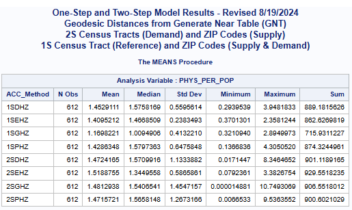
Previous preliminary research has indicated that the one-step physician-to-population ratio (PPR)
or physician-per-population (PYS_PER_POP) mean values
tend to be closer to the statewide mean value
than the mean values from the two-step methods.
The differences are apparent when comparing the means and conducting t-tests and ANOVA.
This additional research is designed to more fully explore and understand why similarities and differences occurr.
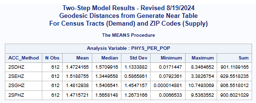
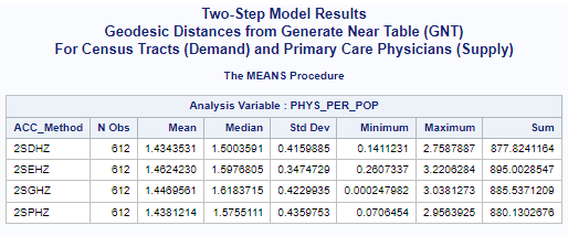
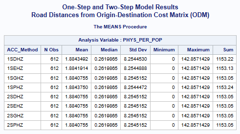
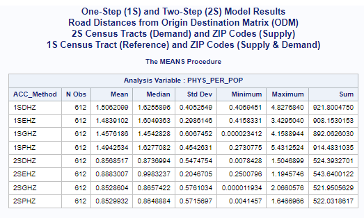
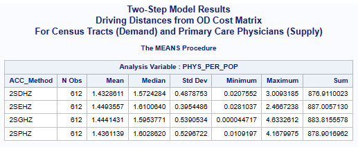
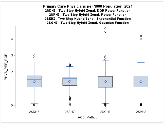
In this case, the statewide mean for primary care physicians per 1,000 population is 1.89336,
calculated for all census tracts (n=612).
There is also an average of 1.45689 physicians per 1,000 population for all census tract.
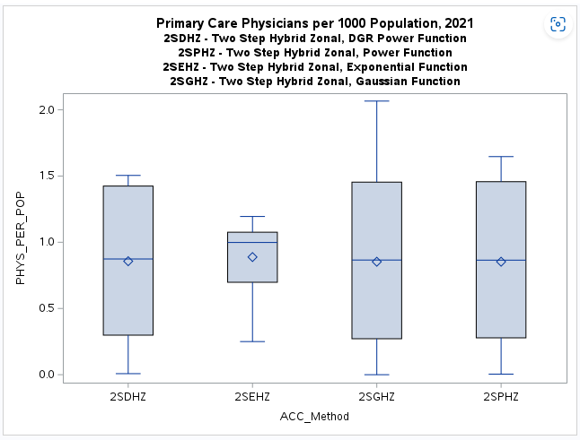
All of the one-step and two-step models (hybrid-zonal rule-based)
with geodesic distances and various distance decay (DGR-power function, exponential, Gaussian, power)
produced very similar results (see table below).
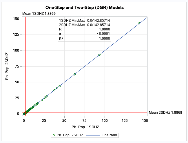
The scatter plot (see below) for the numerical relationship between the one-step and two-step
models using the DGR function graphically shows this similaritay (scatter plots comparing all other
one-step and two-step models are similar).
Note: All models use the hybrid-zonal rule-based function following the guidelines
originally sugested by the New Mexico Legislature (SJM 36, 1996).
One-Step (1S) and Two-Step (2S) Model Results
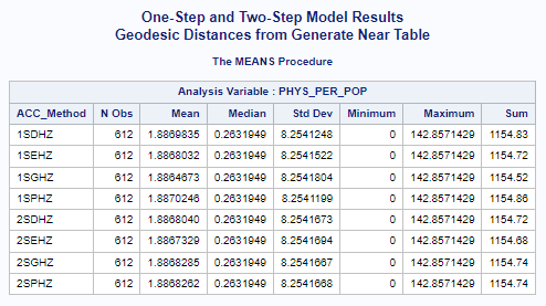
Accessibility Method(ACC_Method): One-Step(1S), Two-Step(2S), DGR-Power(D), exponential(E), Gaussian(G), power(P),
and Hybrid-Zonal(HZ).
This was surprising as some numerical differences between the one-step
and the two-step methods were expected.
These similarities do make sense on closer examination as this phase of the analyses is
based only on census tracts and population weighted centroids.
In otherwords, both the one-step and two-step methods are based on the same
selected data points for both population (demand) and physician (supply) data.
Also both methods are essentially ratio measures of supply to demand.
In this type of application, both methods are composite measures that combine both
the supply of physicians and the population demand for their services.
These numerical results strongly support the similarity of these methods. The textbook by Professor Wang (
Wang 2017; Appendix 5A) provides a statistical/mathematical proof that
shows that "the two-step methods are only a special case of the gravity-based methods".
When appropriate, I will use some additional data science based techniques to help the understanding
of similarities and differences in the resulting data distributions from the various one-step and two-step gravity
based methods (see How to Compare Two or More Distributions).
I will also be learning about and using the new
ArcGIS Pro Data Engineering facility.
See the recent Technical Session from the 2022 Esri Users Conference
(Data Engineering & Visualization for Spatial Data Science) for an excellent introduction.
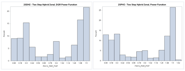
The following maps
are example results of both the one-step (1SDHZ) and two-step methods (2SDHZ) using the hybrid-zonal
rule-based (DGR-power) methods (
PDF,
or see embeded web map below).
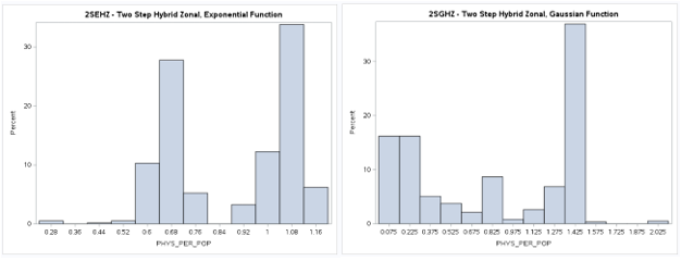
Note that these maps are not exactly similar as some census tracts with
different values were assigned to different map classes or categories.
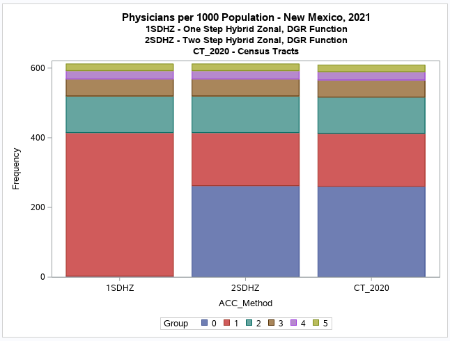
This is apparent for the second category or group (G.1) where the one-step method shows that there appears to be some
accessibility, although relatively low (below the national provider-to-population benchmark of 0.79).
But the two-step method has many of the same census tracts in the first category (G.0) indicating no accessibility.
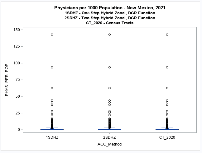
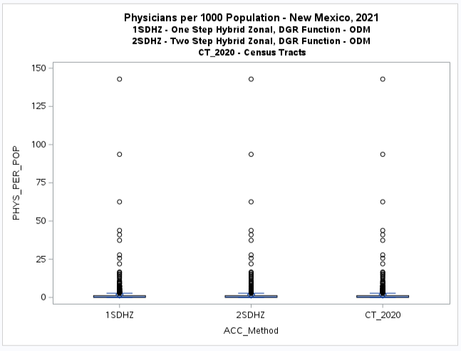
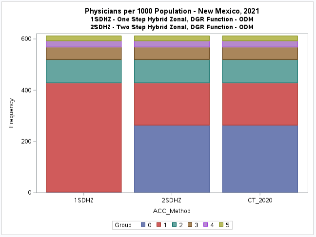
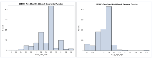
It is difficult to see the difference with a boxplot but the histogram (see below) clearly shows this discrepancy.
It also shows that there is no apparent difference between the
two-step method results and the original values for the census tracts (CT_2020).
The additional map of original values (CT_2020, see below) when compared to the two-step model results (2SDHZ) shows that
the two-step model was more restrained in measuring accessibility for this example application.
This discrepancy, or the tendency of either method to over-estimate or under-estimate accessibility is essentialy
the main focus of this research project.
However, the results based only on census tracts while informative, should be viewed with caution as the two-step method
was not designed to be used this way.
Hopefully the results from the follow-on analyses using ZIP Codes and individual locations will provide a better
understanding of these discrepancies.
Additional Note: The national provider-to-population benchmark for primary care physicians has been revised
in 2019 to 8.9 per 10,000 or 0.89 per 1000 population
(see New Mexico Health Care Workforce Committee 2021 Annual Report, Pg. 32 and
2019 State Physician Workforce Data Report).
I will update my analysis and maps to reflect this. The data I am using for this methodology focused
study is not the official data. It is a overcount that possibly contains many non-practicing, part-time, some physicians that
practice at multiple locations, and perhaps misclassified primary care physicians.
The maps produced by all the other models using geodesic distances and various distance decay methods
also exhibit this discrepancy between the one-step and two-step methods.
A Web Map
using either ArcGIS Experience Builder
or Map Viewer Classic
has been prepared that will facilitate comparing maps.
However there are some differences and additional box plots and scatterplots will be prepared to examine the extent.
These results may demonstrate that no significant numerical differences should be expected using either a one-step or two-step
model when based on a composite (supply and demand) method with provider and population data aggregated to the same geographic
area such as census tracts and calculations based on population weighted centroids.
It may also demonstrate that a composite method tends to result in mean (physician per 1,000 population) values that
are extremly close to the actual mean values per geographic data collection unit such as census tracts.
Further, it may clearly show that the one-step method is the most suited for applications that are based on only one
geographic data collection unit such as census tracts.
View the Web Map in a new tab
Toggle side panel (top left) for Zoom, Layers, and Legend
(Click map feature for pop-up information)
Census Tract Population and ZIP Code Physician Data (GNT)
(Revised 1/7/2023)
Special Note (8/18/2024) : There was an error in the calculation of the
2SEHZ, 2SGHZ, and 2SPHZ (CTZIP GNT) models. They are being recalculated and the affected
graphics and web maps are being redone.
In order to better evaluate the results the series of one-step and two-step models have been prepared using
ZIP Codes (see United States ZIP Code Boundaries 2021,
U.S. ZIP Code Points and
ZIP Code Population Weighted Centroids - HUD)
instead of census tracts for physician locations.
The same distance decay functions (DGR-power, power, exponential, and Gaussian) have been applied,
all with the same hybrid-zonal rule-based method but with physician locations aggregated
to ZIP Codes.
Separating the population (demand by census tracts) from
the physicians (supply by ZIP Codes) may allow for the difference between the one-step and two-step
methods to become more noticeable.
Also any advantages or disadvantages of the two-step methods in comparison to the one-step
methods may be apparent.
Update (7/30/2023): One-step models are currently being prepared to allow for
the comparison of results. The two-step model results will not change.
My previous one-step model applications and research had only used a single geographic unit such as census tracts
or ZIP Codes for the aggregation of both population and physician data.
This research will experiment with the application of the one-step method using two geographic units (census tracts and ZIP Codes).
Note that the one-step method is a composite method that incorporates both supply and demand.
A one-step method can be constructed with just census tracts or ZIP Codes or with the both.
If the same geographic units are used, both supply (physicians) and demand (population) are aggregated to that area.
However, if two different geographic units are used, one unit are just reference locations (ex. Census Tracts) and
the supply (physicians) and demand (population) are in the other units (ex. ZIP Codes).
The one-step results presented her use census tracts as reference units and for displaying results while the
ZIP Codes have aggregated supply (physicians) and demand (population).
Note that this can be reversed where ZIP Codes can be used for reference locations and census tracts
can have aggregated supply (physicians) and demand (population). I do not plan to use this configuration now or
to just use only ZIP Codes as I have done in the past unless necessary to facilitate comparisons.
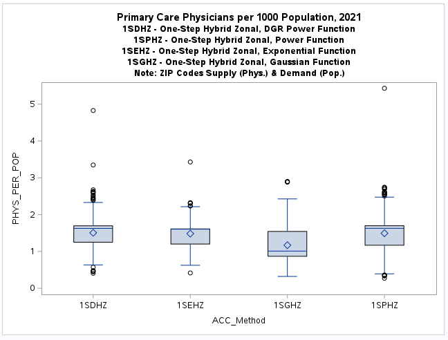
One-Step (1S) Model Results
This experimental model configuration is presented as an example of how reasonable results can be obtained
from various gravity model derivations. The boxplots and histograms along with the resulting
web map
exhibit the tendency of the one-step models to more evenly spread the results as opposed to the two-step models
that have a tendency to be more concentrated or skewed in this census tract and ZIP Code application.
This discrepancy, or tendency of either method (one-step or two-step) to over-estimate or under-estimate
accessibility is a major focus of this research project.
It may be possible to directly statistically compare these models to get a better understanding, although
the different way they were configured is problematic.
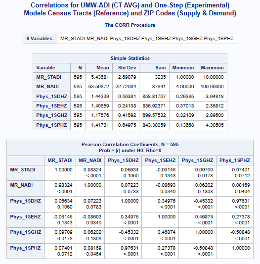
The preliminary correlations (see above) with the
UMW Area Deprivation Index (ADI)
data shows a very weak negative correlation for the exponential model
and suprisingly very weak positive correlation for the other distance decay models.
Further indirect comparisions (see Model Comparisons sections below) using various health disparities
and social determinants of health are planned and may help evaluating this research question.
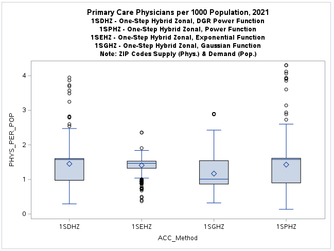
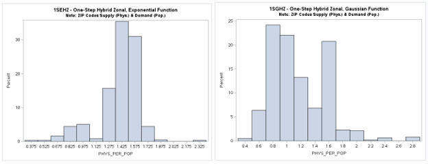
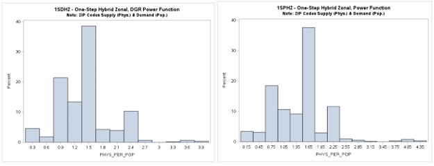
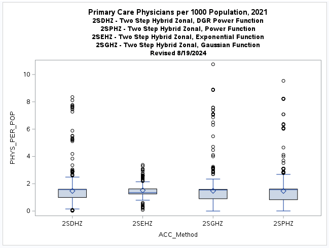
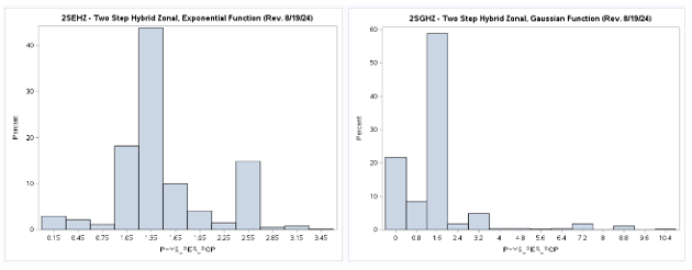
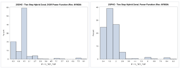
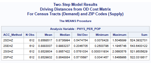
Two-Step (2S) Model Results (Revised 8/19/2024)
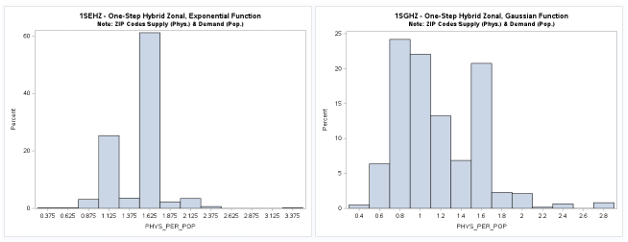
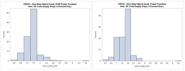
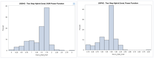
A table of descriptive statistics, selected boxplots and a histogram (below) clearly summarize the results.
There is a obvious difference in the shape of the two-step distribution when using the exponential (2SEHZ) distance
decay method compared with the other distance decay methods (2SDHZ - DGR Power, 2SGHZ - Gaussian, and
2SPHZ - power) shown by the boxplots (below). The histograms (below) clearly shows that the exponential distance decay
method produces diffrently distributed results along with a mean value (see table) that is islightly greater than the
statewide average (1.45689) but lower than the mean (1.89336) plus a much lower maximum value (~3.38) than the others.
The other distance decay methods have similar mean values closer to the statewide average and somewhat similar maximum
values (>= 8.34). This may indicate that
the choice for either a one-step or a two-step model should also consider the selection of
the most appropriate distance decay function. However, more direct comparisons of the one-step and two-step
model results are needed to determine if there are any significant differences in the results. An additional
section of this study will present these comparisons (see below).
Special Note (8/18/2024) : There was an error in the calculation of the
2SEHZ, 2SGHZ, and 2SPHZ (CTZIP GNT) models. They are being recalculated and the affected
graphics and web maps are being redone.
Accessibility Method(ACC_Method): Two-Step(2S), DGR-Power(D), exponential(E), Gaussian(G), power(P),
and Hybrid-Zonal(HZ).
Revised (8/20/2024):
The web map (below) allows for a visual comparison of the various two-step models with different
distance decay functions.
The DGR power (2SDHZ), Power (2SPHZ), and Gaussian (2SGHZ) distributions and maps are similar
and may properly portray the concentration of physicians in relation to population.
However the exponential distribution and map are different (see histograms and boxplots above).
The exponential model may actually provide more realistic results by
more evenly distributing physician accessibility, but the potential to over-predict
in locations without enough physicians needs further evaluation.
View the Web Map in a new tab
Toggle side panel (top left) for Zoom, Layers, and Legend
(Click map feature for pop-up information)
Census Tract Population and Individual Physician Locations (GNT)
This is the classic configuration for the application of the two-step models. It requires many more
distance measurments and calculations which can be prohibitive when using roadway distances due to
increased costs from commercial providers. This is not a problem when using geodesic distances.
The same series of two-step models using various distance decay functions
(DGR-power, power, exponential, and Gaussian) have been prepared.
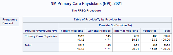
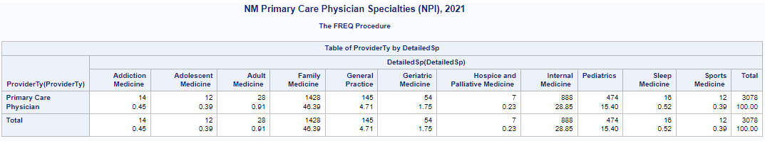
There are 3,078 individual primary care physician locations (Provider Type = 'Primary Care Physician')
that will have been used for this phase of
the analysis that were previously aggregated to census tracts or ZIP Codes.
Two-Step (2S) Model Results
Accessibility Method(ACC_Method): Two-Step(2S), DGR-Power(D), exponential(E), Gaussian(G), power(P),
and Hybrid-Zonal(HZ).
View the Web Map in a new tab
Toggle side panel (top left) for Zoom, Layers, and Legend
(Click map feature for pop-up information)
Problems Encountered (GNT)
I have had some minor problem using the Census Bureau's population weighted centroids for census tracts
(see Centers of Population). Some of these centroids fall outside of the actual
census tract polygons. This file may have been prepared
using a Spatial Join resulting in some (n=17 of n=612) duplicate IDs (GEOID20, etc.)
acquired from a nearby census tract. I had to do some manual edits in
ArcGIS Pro to correct this problem.
I used SAS
to merge together the datasets derived from the ArcGIS Pro
Generate Near Table (GNT) and other tools.
These files contained the number of providers and population
plus the population weighted center points used to create the GNT. All files had a census tract's unique
identification (GEOID20) and numeric equivalent (GEOIDN) generated by SAS. A seried of ArcGIS Pro
joins will be used to prepare the maps.
Update (12/6/2022):
I have also found some minor problems with the
ZIP Code Population Weighted Centroids - HUD data.
There are 20 mislocated (0,0 - Longitude, Latitude -
Null Island) centroids
for the 343 ZIP Code polygons.
Unfortunately I only noticed this when creating an O-D Cost Matrix using credits
from ArcGIS Online for road distances between census tracts and ZIP Codes.
I have used the ArcGIS Pro
Feature To Point Tool to calculate centroids for these ZIP Codes to use
as replacements for the missing population weighted centroids.
However I will need to redo the previous analyses that used geodesic distances for ZIP Codes.
I have prepared a revised
Generate Near Table (GNT) for this update.
Hopefully the results will not be very different, but it will take more time.
Update (1/4/2023):
The revised Generate Near Table (GNT) has been prepared and the results for the two-step model comparisions
using census tract population and ZIP Code physician data have been redone (see above). There were more difference
than expected. The choice of an appropriate distance decay function seems to be the most important consideration.
Special Note (8/21/2024): There was an error in the calculation of the
2SEHZ, 2SGHZ, and 2SPHZ (CTZIP GNT) models. They have been recalculated and the affected
graphics and web maps have been redone.
Note: All initial results are being derived using SAS.
Previously developed Python
and R scripts will be updated
later to check and compare results.
Plus both
Jupyter Notebooks and
ArcGIS Pro Notebooks
will be prepared for others to review. These notebooks will contain additional graphics.
Road Network Distance Based Analyses (ODM)
I will use ArcGIS Pro
to prepare a OD Cost Matrix Analysis Layer to obtain road distances and drive times
for 2020 NM census tract population weighted centroids, ZIP Code centroids, and individual physician locations.
ArcGIS Online provides a convenient routing service for use with ArcGIS Pro
(see Network analysis using routing services).
However, I hope to eventually use ArcGIS StreetMap Premium.
I will be exploring the possibility of cost sharing with others at UNM or those at NM state government agencies who have already
prepared or plan on preparing this resource for similar research projects.
Census Tracts for both Population and Physician Data (ODM)
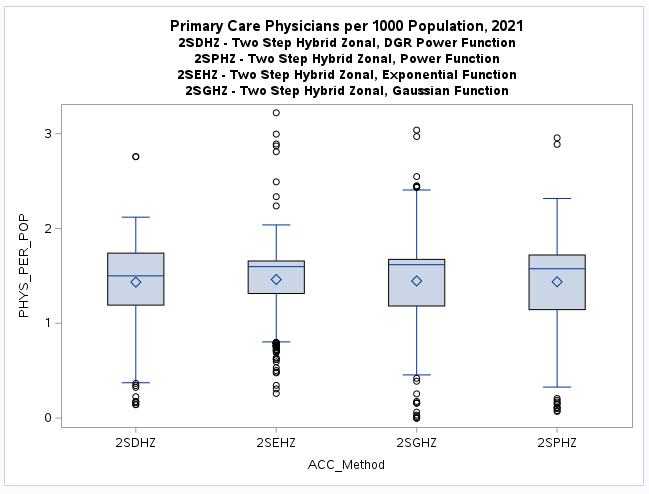
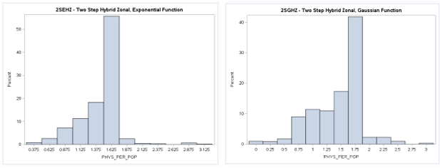
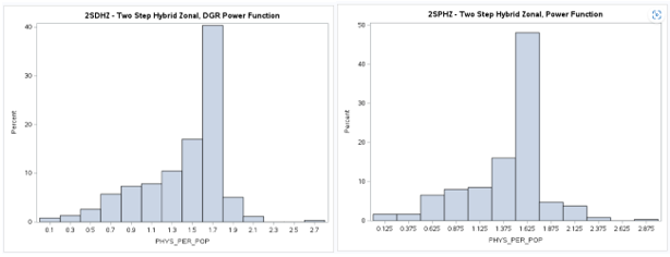
Note: A complete OD Cost Matrix (ODM) was recently obtained (5/18/2023) and results are now avilable.
These results are very similar to those previously obtained from the census tract
to census tract models using a GNT instead of a ODM.
I am still somewhat surprised by these results and they should still be regarded as preliminary.
I will be checking them using Python scripts and R code that I have developed that need further modifications
and careful review for these specific model applications.
These results, when verified, may be useful to evaluate how various configurations of geographic access
gravity models are related to established measures of health inequality (health disparities)
and social determinants of health (
SDOH).
Some preliminary results are already available (see One-Step and Two-Step Model Comparisons) below.
Additional Note: The national provider-to-population benchmark for primary care physicians has been revised
in 2019 to 8.9 per 10,000 or 0.89 per 1000 population. This benchmark has been used here as in all the gravity model
analyses comparisions except for the census tracts for both population and physician data (GNT) that uses the previous
benchmark of 0.79 (see above). However there is not much difference in the results and graphics (charts and
web maps) that have been provided. There are some small observable differences in the mean and standard deviation
values (see tables) that interestingly shows how similar results have been obtained using either a GNT and ODM for distance.
The provided web map only includes the results for the one-step and two-step
DGR-Power and Gaussian distance decay functions that illustrates the important aspect previously noted for the GNT based analysis.
For the DGR-Power function the two-step model has many zero valued census tracts (G.0) while the one-step model does not (G.1).
This discrepancy, or tendency of either method (model) to over-estimate or under-estimate accessibility is a major focus
of this research project.
One-Step (1S) and Two-Step (2S) Model Results
Accessibility Method(ACC_Method): One-Step(1S), Two-Step(2S), DGR-Power(D), exponential(E), Gaussian(G), power(P),
and Hybrid-Zonal(HZ).
View the Web Map in a new tab
Toggle side panel (top left) for Zoom, Layers, and Legend
(Click map feature for pop-up information)
Census Tract Population and ZIP Code Physician Data (ODM)
Update: (1/7/2023 - 1/22/2023)
I have prepared an ArcGIS Pro
OD Cost Matrix Analysis Layer (ODM) to obtain road distances and drive times
for 2020 NM census tract population weighted centroids and 2021 ZIP Code population weighted centroids.
Update (7/30/2023): One-step models are currently being prepared to allow for
the comparison of results. The two-step model results will not change.
My previous one-step model applications and research had only used a single geographic unit such as census tracts
or ZIP Codes for the aggregation of both population and physician data.
This research will experiment with the application of the one-step method using two geographic units (census tracts and ZIP Codes).
Note that the one-step method is a composite method that incorporates both supply and demand.
A one-step method can be constructed with just census tracts or ZIP Codes or with the both.
If the same geographic units are used, both supply (physicians) and demand (population) are aggregated to that area.
However, if two different geographic units are used, one unit are just a reference locations (ex. Census Tracts) and
the supply (physicians) and demand (population) are in the other units (ex. ZIP Codes).
The one-step results presented her use census tracts as reference units and for displaying results while the
ZIP Codes have aggregated supply (physicians) and demand (population).
Note that this can be reversed where ZIP Codes can be used for reference locations and census tracts
can have aggregated supply (physicians) and demand (population). I do not plan to use this configuration now or
to just use only ZIP Codes as I have done in the past unless necessary to facilitate comparisons.
One-Step (1S) Model Results
This experimental model configuration is presented as an example of how reasonable results can be obtained
from various gravity model derivations. The boxplots and histograms along with the resulting
web map
exhibit the tendency of the one-step models to more evenly spread the results as opposed to the two-step models
that have a tendency to be more concentrated or skewed in this census tract and ZIP Code application.
This discrepancy, or tendency of either method (one-step or two-step) to over-estimate or under-estimate
accessibility is a major focus of this research project.
It may be possible to directly statistically compare these models to get a better understanding, although
the different way they were configured is problematic.
The preliminary correlations (see above) with the
UMW Area Deprivation Index (ADI)
data shows very weak negative correlations and suprisingly
a very weak positive correlation for the Gaussian distance decay model.
Further indirect comparisions (see Model Comparison sections below) using various health disparities
and social determinants of health are planned and may help evaluating this research question.
Two-Step (2S) Model Results
A table of descriptive statistics, selected boxplots and a histogram (below) clearly summarizes the results.
The web map (below) allows for a visual comparison of the various two-step models with different
distance decay functions.
There is a noticeable difference in the shape or form of the resulting distributions
(more bimodal) when road distance
from an ODM are used compared with geodesic distances from a Generate Near Table (GNT).
The maps of the spatial distribution of results are also noticeable different with prominent
concentrations in urbanized areas having higher population density.
The exponential distance decay function is clearly somewhat different (more bimodal and less dispersed)
with more census tracts below the national provider-to-population benchmark of 0.89 than the other
distance decay functions.
It is very interesting that all the mean values are similar and close to the national benchmark (0.89)
but this should be viewed with extreme caution.
This is not an official count of practicing physicians (see
NM Healthcare Workforce Committee
2022 Annual Report)
and contains many that are part-time, retired, and possible duplicate entries for those that practice
at multiple locations.
However, the problem of deciding which distance decat function provided the most realistic pattern
is not resolved.
Subsequent research statistically comparing these results to measures of health inequalities (health disparities)
is planned (see below) that may help deciding the choice of the most appropriate distance decay function.
Accessibility Method(ACC_Method): Two-Step(2S), DGR-Power(D), exponential(E), Gaussian(G), power(P),
and Hybrid-Zonal(HZ).
View the Web Map in a new tab
Toggle side panel (top left) for Zoom, Layers, and Legend
(Click map feature for pop-up information)
Census Tract Population and Individual Physician Locations (ODM)
Update (6/2/2023): Some problems resolved and results are available
This is the classic configuration for the application of the two-step models.
It requires many more distance measurments and calculations.
The costs when using commercial providers of street data road networks is expensive
and not in the budget for this class project.
Fortunately UNM like other universities has a
Esri Higher Education Site License
for academic uses.
I have received assistance from
UNM's Earth Data Analysis Center (EDAC)
to prepare an Origin Destination Matrix (ODM) for this
phase of the analyses and a complete ODM has been recently obtained (5/18/2023).
A minor problem (1,000 record limit) was previously encountered when attempting to create this ODM.
As there are 3078 physician locations, it was decided to create four separate
feature layers and generate four smaller ODMs that can be combined into the larger required
ODM for creating the models.
I had some problems (data merging issues)
combining the separate pieces and generating the 2SFCA models.
I solved these problems (5/28/2023) that are mostly due to repeat of the Destanat_1 item
values in the ODM that had to be created in four separate pieces.
Note: In 1984 both DGR and EDAC (previously the Technology Application
Center - TAC) cooperated to acquire a site license for
Esri's Arc/Info
and were among the first 100 users worldwide. This license has since evolved
into a statewide educational license providing access to Esri software
for New Mexico's universities.
Two-Step (2S) Model Results
Results for the various 2SFCA models are now available below (6/2/2023).
The mean values are again very similar as is the general shape of the distributions as shown
by the histograms. However the box plots reveal that there are now more outliers than in the
previous models that used ZIP Code weighted centroids for the physician (supply) locations.
The exponential model also seems to be more compact as before with a smaller range of values.
However, these results should be viewed with caution as
this is not an official count of practicing physicians (see
NM Healthcare Workforce Committee
2022 Annual Report)
and contains many that are part-time, retired, and possible duplicate entries for those that practice
at multiple locations.
Again the problem of deciding which distance decay function provided the most realistic pattern
is not resolved.
Subsequent research statistically comparing these results to measures of health inequalities (health disparities)
is planned (see below) that may help deciding the choice of the most appropriate distance decay function.
Accessibility Method(ACC_Method): Two-Step(2S), DGR-Power(D), exponential(E), Gaussian(G), power(P),
and Hybrid-Zonal(HZ).
View the Web Map in a new tab
Toggle side panel (top left) for Zoom, Layers, and Legend
(Click map feature for pop-up information)
Problems Encountered (ODM)
As noted in the GNT problem section I found some minor problems with the
ZIP Code Population Weighted Centroids - HUD data.
There are 20 mislocated (0,0 - Longitude, Latitude -
Null Island) centroids
for the 343 ZIP Code polygons.
Unfortunately I only noticed this when creating an O-D Cost Matrix using credits
from ArcGIS Online for road distances between census tracts and ZIP Codes.
I have used the ArcGIS Pro
Feature To Point Tool to calculate centroids for these ZIP Codes to use
as replacements for the missing population weighted centroids.
The 1,000 record limit for origins and destinations (see
Generate Origin Destination Cost Matrix) requited spliting the physician feature
layer (n=3078) into four separate feature layers. Four ODMs were produced and then merged back
together as the larger necessary ODM for creating the models.
I had some problems (data merging issues)
combining the separate pieces and generating the 2SFCA models.
I solved these problems (5/28/2023) that are mostly due to repeat of the Destanat_1 item
values in the ODM that had to be created in four separate pieces.
Note that when creating a numeric GEOID variable for merging it should be derived from GEOID20 not FIPS
as FIPS does not contain all the new 2020 census tracts (duplicate records for the split census tracts).
In the future if some funding for this research is available using
ArcGIS Street Map Premium would be more efficient and produce a more accurate and up-to-date ODM.
For New Mexico there were only 600 of the 612 census tracts with valid data for the
Social Vulnerability Index (SVI).
This is because some census tracts contain group quaters (dormitories, prisons, etc.) where the population was not counted.
Also for the United States the
Area Deprivation Index (ADI)
is available only at the census block group or ZIP Code (ZCTA?) levels of geography.
I was able to aggregate the census block groups to census tracts and used the average (MR - rounded mean) value of
the block groups that composed the census tracts. There were 595 of the 612 census tracts that contained valid data
as some block group data were suppressed (low population or housing group quarters).
However these results should be viewed with caution as there is a potential for statististical bias and excessive
variation due to the MAUP.
Note: All initial results are being derived using SAS.
Previously developed Python
and R scripts will be updated
later to check and compare results.
Plus both
Jupyter Notebooks and
ArcGIS Pro Notebooks
will be prepared for others to review. These notebooks will contain aditional graphics.
I will need to use an open source Python package
(SASPy)
that allows for data exchange between SAS and
Pandas dataframe objects.
I have encountered some recent problems getting SASPy
to work with Jupyter Notebook in both
ArcGIS Pro
and Anaconda.
The fix I eventually found requires downloading and installing additional
encryption jar files.
I have posted this problem and a solution on the
Esri Community website.
One-Step and Two-Step Model Comparisons
Some Preliminary Results
A comprehensive comparision of the results of the one-step and-two-step models with standard statistical methods
(t-tests and ANOVA) plus addiditional
exploratory data analysis (eda)
and exploratory spatial data analysis (esda)
techniques is being prepared
(
Geographic Acces to New Mexico Health Care Providers and Facilities - analyses page).
It is possible that the one-step and two-step models produce very similar results and there
are no distinct advantage of either. The availability of data and how the models are configured (separation of supply and demand)
plus the type of distance-decay function may be the main factors contributing to
any appreciable differences.
Addressing the tendency of various models to over-predict or under-predict is a more difficult problem that needs to be investigated.
The results from these geographic access models can be compared to measures of health inequality (health disparities) to statistically
evaluate the relationships.
I plan to conduct further spatial statistical analyses
using methods such as geographically weighted regression.
(GWR)
and the recently developed multiscale geographically weighted regression
(MGWR).
These spatial methods will be useful to see how results from the geographic access gravity models
are related to various measures of health inequality (health disparities)
and social determinants of health (
SDOH).
For instance, several methods to classify rural or urban census tracts
(see Rural Definitions for Health Policy and
Rural-Urban New Mexico, Healthcare Access)
have been developed.
Plus the CDC has a well developed Social Vulnerability Index (SVI)
for census tracts.
Also a neighborhood Area Deprivation Index (ADI)
for census block groups is available and
there is a recently developed R package geomarker-io
that can be used to calculate a community deprivation index (CDI)
using the Census Bureau's American Community Survey
(ACS) census tract data.
Another potentially useful resource is the
Climate and Economic Justice Screening Tool (Justice 40).
These classifications and other socio-economic and demographic attributes used to identify
Health Professional Shortage Areas (HPSAs)
and Medically Underserviced Areas (MUAs)
will be evaluated as possible components of several spatial statistical models
(see Esri Spatial Statistics Resources).
I am currently researching the possibility of developing a composite index/indicator (see
Esri Technical Paper and
Calculate Composite Index Tool (Spatial Statistics))
from the spatial combination of these data sources.
However, these previously developed incices are at different levels of geography (counties, census blocks or tracts) and many are based on
the Census Bureau's American Community Survey (ACS)
and are currently only available for 2010 census geography.
It may be better to develop similiar indices for subsequent analyses that will include more recent data from the
2020 census as it is made available from the Census Bureau
at the census tract and block group geographic levels.
Recent census data will also be available for
geoenrichment
from Esri's
ArcGIS Living Atlas
using the
Data Enrichment
service and these recent data have been used to develop their Socioeconomic Status Index
(SEI).
The preliminary results at this point indicate that model configuration and choice of distance decay function strongly influence results.
A one-step model with only data (supply and demand) available at census tracts can produce reasonable results as long as
an appropriate distance decay function is used. A two-step model with the data separated (supply and demand) at different geographic
data collection units (population at census tracts and physicians at ZIP Codes) can also produce reasonable results.
However, using geodesic distances instead of road distances can result in questionable results over long distances at the statewide level.
Further, a more gradual distance decay function may actually provide more realistic results but the potential to over-predict
in less accessible locations needs further evaluation. Hopefully the subsequent analyses using road distances will provide a clearer
understanding of how to select an appropriate model for use at a statewide geographic level.
Census Tracts for both Population and Physician Data 1SHGM and 2SFCA Model Comparisons
The tables presented above for population (demand) and physicians (supply) both for census tracts using GNT or ODM distances
clearly show how similar the results from models with various distance decay functions (DGR, exponential, Gaussian, and power)
are. Correlations between just the DGR and Gaussian one-step and two-step models were performed (see below) to illustrate this.
Additional correlations were performed with the UWM-ADI data to evaluate the strength of any relationship. The tables (see below)
clearly show how weak this relationship is. These results suggest that using only census tracts as the basis for these models
would apprently not be the best alternative.
I also suspect that using only ZIP Codes as I have done previously (the original DGR 2002 model) may also not have provided the
best possible results.
However as the one-step models are based on using the same geographic unit, more research should be done before discounting
the utility of this composite measure in favor of the two-step models.
I will be developing updated and more reliable measures of health inequalities and disparities for New Mexico and this preliminary
analyses will be redone to see if the results change.
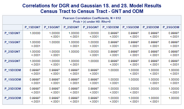
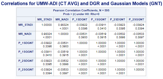
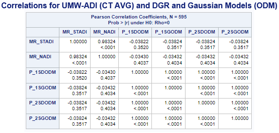
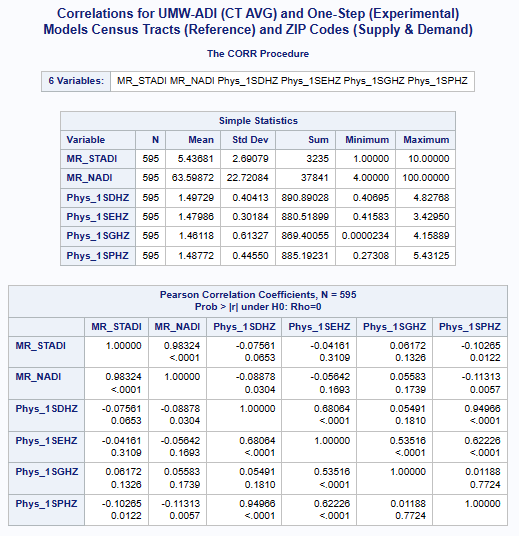
Variables ADI(*MR-Mean Rounded) & (ACC_Method): MR_STADI (State ADI), MR_NADI (National ADI),
One-Step(1S), Two-Step(2S), DGR-Power(D), exponential(E), Gaussian(G), power(P), and Hybrid-Zonal(HZ).
Census Tract (Population) and ZIP Code (Physician) 2SFCA Model Comparisons
Some additional statistical analysis results are now available that compare the 2SFCA gravity model results
(CT Pop. and ZIP Code Phys. with ODM) to both the
Social Vulnerability Index (SVI)
and the Area Deprivation Index (ADI).
A selected portion of these results (see below) suggest that further work to develop a composite index/indicator
plus using methods such as geographically weighted regression
(GWR)
and the recently developed multiscale geographically weighted regression
(MGWR)
could prove useful.
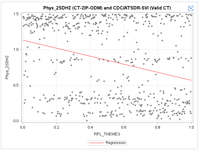
However, the correlations between the 2SFCA gravity model results and both the SDI and ADI
show weak correlations but expected negative relationships.
As the physician-to-population ratio (PPR) increases the severity of both the SVI and ADI decrease but increase
as the PPR is lower.
Although the correlations are weak, it is interesting to note that the 2SFCA gravity models that use the power
based distance decay functions (2SPHZ and 2SDHZ) are slightly greater than both the gravity models that use
the Gaussian (2SGHZ) and the exponential (2SEHZ) distance decay functions.
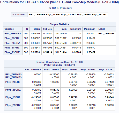
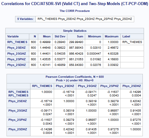
Variables SVI & (ACC_Method): RPL_THEMES (Summary Ranking), Two-Step(2S), DGR-Power(D), exponential(E), Gaussian(G), power(P),
and Hybrid-Zonal(HZ).
View the NM SVI Web Map in a new tab
Toggle side panel (top left) for Zoom, Layers, and Legend
(Click map feature for pop-up information)
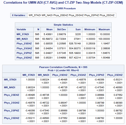
Variables ADI(*MR-Mean Rounded) & (ACC_Method): MR_STADI (State ADI), MR_NADI (National ADI),
Two-Step(2S), DGR-Power(D), exponential(E), Gaussian(G), power(P), and Hybrid-Zonal(HZ).
View the NM ADI Web Map in a new tab
Toggle side panel (top left) for Zoom, Layers, and Legend
(Click map feature for pop-up information)
Census Tract (Population) and Geocoded Physician 2SFCA Model Comparisons
Some additional statistical analysis results are now available that compare the 2SFCA gravity model results
(CT Pop. and Geocode Phys. with ODM) to both the
Social Vulnerability Index (SVI)
and the Area Deprivation Index (ADI).
A selected portion of these results (see below) indicate that the correlations are even weaker than those obtained
when the physician locations were aggregated to ZIP Codes (see above).
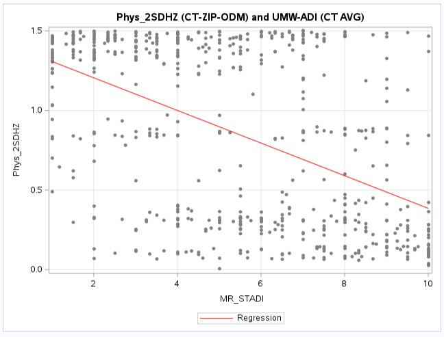
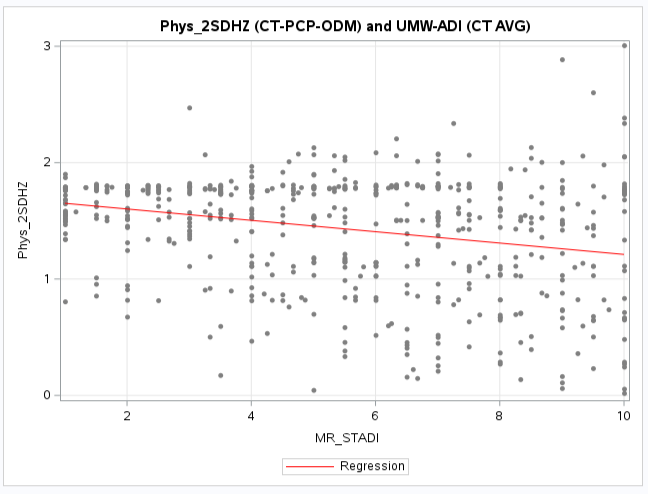
It is interesting to note that for the UWM-ADI comparisons the 2SFCA gravity models that use the DGR power
based distance decay functions (2SDHZ) has a slightly greater corelation than the other gravity models.
However the exponential (2SEHZ) distance decay functions is now the closest correlation value instead
of the power (2SPHZ) as when physicians were aggregated to ZIP Codes.
The same relationship of correlation coefficients (although weaker) is apparent for the SVI comparisons.
These results (see below) also suggest that further work to develop a composite index/indicator plus
using methods such as geographically weighted regression
(GWR)
and the recently developed multiscale geographically weighted regression
(MGWR)
could prove useful and may result in stronger relationship to indices of health disparities.
Variables SVI & (ACC_Method): RPL_THEMES (Summary Ranking), Two-Step(2S), DGR-Power(D), exponential(E), Gaussian(G), power(P),
and Hybrid-Zonal(HZ).
View the NM SVI Web Map in a new tab
Toggle side panel (top left) for Zoom, Layers, and Legend
(Click map feature for pop-up information)
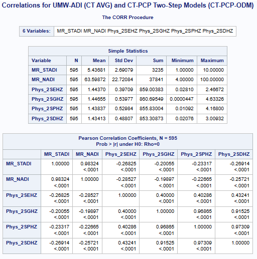
Variables ADI(*MR-Mean Rounded) & (ACC_Method): MR_STADI (State ADI), MR_NADI (National ADI),
Two-Step(2S), DGR-Power(D), exponential(E), Gaussian(G), power(P), and Hybrid-Zonal(HZ).
View the NM ADI Web Map in a new tab
Toggle side panel (top left) for Zoom, Layers, and Legend
(Click map feature for pop-up information)
Future Comparisons
Further comparisions using other availible indices (such as the MUA, CDI, and NDI) plus
similar indices derived from 2020 census data at the tract level of geography are being prepared.
I am currently researching the possibility of developing a composite index/indicator (see
Esri Technical Paper and
Calculate Composite Index Tool (Spatial Statistics)) based on aspects of these well-developed indices.
A more detailed discussion will be available as more of these analyses are conducted
and I obtain some help interpreting the results from other researchers with
public health and stronger statistical backgrounds.
Future research may indicate that there is a counter-intuitive way of interpreting the poor
correlations with health care inequality and disparity indices plus social determinants of health.
These results may actually indicate how out-of-balance the distribution of primary care physicians actually is in New Mexico.
The various models and their correlations may be useful to show and illustrate a range of statewide geographic accessibility
from poor (weak) to somewhat better (stronger).
Note: Other potentially useful indexes are the community deprivation index (CDI) that can be calculated using
a recently developed R package geomarker-io
and the CDC's Neighborhood Deprivation Index
(NDI).
Both can be calculated with R and there is a
R package tidycensus that can be used.
Several Esri products can also be used to acquire and enhance recent census data
(see Esri Data Enrichment).
I am currently working with these resources and hope to have results for 2020 New Mexico census tracts as
the necessary data are made available from the Census Bureau.
After an appropriate model is selected and more recent population and verified physician data are available, it would be possible to employ
this model using other geographic data collection and political geographic areas.
For instance, NM Small Areas
that contain a wealth of health related data could be supplemented by these higher resolotion geographic accessibility measures.
Also New Mexico State Legislative (House and Senate) districts could perhaps be the focus of a follow-on study using an appropriate model.
(See GIS Voting District Data).
This could be helpful for legislators to get a better picture
of any disparities that may affect their constituents.
I'm also very interested in comparing the one-step and two-step gravity models for evaluating geographic accessibility to retail locations.
My previous research (Albuquerque Food Retail Locations and Food Deserts)
used a one-step gravity model but a two-step model could prove more useful for this type of application.
Update: (9/3/2023):
The results presented so far have contained mostly descriptive statistics and preliminary data visualizations and analyses using SAS.
An additional analyses focused web page is being prepared
(
Geographic Acces to New Mexico Health Care Providers and Facilities - analyses page).
that will develop appropriate social and health care inequality and disparity indices
and conduct further standard and spatial statistical analyses.
SAS will continue to be used as it is very helpful for data engineering (data preparation, integration, and wrangling)
and standard statistical analyses.
The SAS OnDemand for Academics
resource has also been invaluable for processing larger data sets very quickly.
A transition to using Python and R will be made during this next phase of work that will include various
spatial statistical methods.
Some of the models will be recalculated using ArcGIS Pro script tools and Python notebooks that will include
statistical methods.
These computing resources will eventually be made available for other researchers to use and modify.
Mixed Model Analyses
Depending on the results of the comparisions of the one-step and two-step gravity model methods,
the results may indicate that
a particular model may be more suitable and potentially useful for a statewide (combined rural and urban)
application and another more suitable and potentially useful for separate
urbanized areas and their more populated surroundings.
A mixture of geodesic distances and
road network distances or travel times may be evaluated if the results indicate potential utility.
Selected Links and Publications
I recently prepared a literature review and a very brief
power point class presentation
for Geography 601 (Intro to Geographic Theory and Application, Fall 2021).
I will be providing a link to some of the publications and web resources I found useful.
As this is an ongoing research project, I will include some additional more recent items in the future.
Address and Contact Information
     Larry Spear, Sr. Research Scientist (Ret.)
     Division of Government Research
     University of New Mexico

     Email: lspear@unm.edu  lspearnm@gmail.com
     WWW: https://www.unm.edu/~lspear
     LinkedIn https://www.linkedin.com/in/larry-spear-93371970
 UNM's Home Page
Last Revised: 8/21/2024 Larry Spear (lspear@unm.edu)